Shading

This page documents how SunPeek handles shading effects on collector arrays. Shading impacts both the direct (beam) and the diffuse radiation reaching the collectors. These three types of shading can be distinguished:

• External shading: Shadows cast by objects outside the collector field, such as buildings, trees, or terrain features (mountains, hills).

• Internal shading: Row-to-row shading within the collector field, where the front collector row casts shadows on the rear rows.

• Diffuse masking: The reduction of diffuse sky radiation due to view obstruction by the front collector row.

The virtual sensor is_shadowed on each Array indicates whether the array is considered shaded at any given timestamp. This sensor combines information from external shading (minimum sun elevation, user-provided shadow data) and internal shading calculations. It is used, for example, in Power Check to fulfill the criterion to exclude shaded data.

See also

For a comprehensive explanation of shading, see section A.6 in Guide to ISO 24194:2022 Power Check.

External Shading

External shading refers to shadows from objects outside the collector field. ISO 24194 does not specify how to treat external beam shading, but SunPeek offers two approaches.

User-Provided Shadow Masks

Through the Python API, users can provide their own shadow information for each collector field. This is useful when horizon profiles or detailed 3D shading analyses have been performed using external tools (e.g., OpenSolar, Solargis, or PVGIS).

To use custom shadow information, assign a sensor to the is_shadowed slot of an Array. When a user-provided sensor is assigned, SunPeek uses this data directly instead of calculating shading internally.

See the Array API documentation for details.

Minimum Sun Elevation

A practical approach to exclude external shading is to define a minimum sun elevation angle \(\theta_{\min}\). When the sun’s apparent elevation falls below this threshold, the array is considered shaded. This simple parameter can effectively exclude times when mountains, buildings, or other obstacles on the horizon cast shadows on the collector field (see figure below).

This parameter can be set:

• Via the Web UI during plant configuration in the Array input form (field: “Sun Minimal Elevation”)

• Via the Python API as the min_elevation_shadow parameter on Array

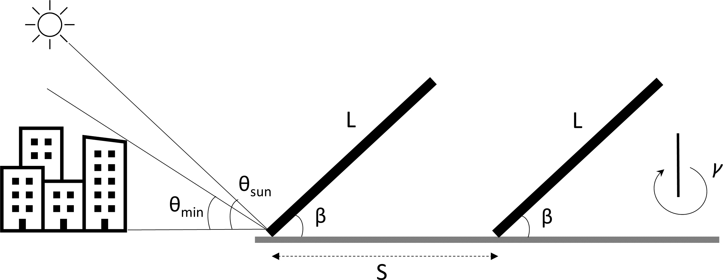
Collector field geometry illustrating the minimum sun elevation angle approach to exclude external shading from obstacles on the horizon.

Internal Shading

Internal shading (row-to-row shading) occurs within regularly arranged collector arrays when the front collector row casts shadows on the rear rows. SunPeek calculates internal shading automatically based on the collector field geometry: tilt angle \(\beta\), azimuth \(\gamma\), collector gross length \(L\), and row spacing \(S\).

SunPeek assumes uniformly arranged arrays and uses different algorithms depending on whether the collector azimuth matches the ground azimuth.

Note

Internal shading calculation for one-axis and two-axis tracking collectors is not yet implemented. The current algorithms apply to fixed-mounted collectors only.

Bany-Appelbaum Algorithm (Flat or Same-Azimuth Ground)

For the common case where collector azimuth equals ground azimuth (\(\gamma_c = \gamma_g\)), including flat ground (\(\theta' = 0\)), SunPeek uses the classic Bany-Appelbaum algorithm [BanyAppelbaum1987] as described in ISO 24194, Section 5.5.

The algorithm calculates the shading fraction based on:

• Sun position (azimuth and elevation)

• Collector geometry (tilt, gross length, row spacing)

• Ground tilt in the collector azimuth direction

API: calc_BanyAppelbaum_shading()

Sloped Ground Algorithm (Different Azimuths)

For the more general case where collector azimuth differs from ground azimuth (\(\gamma_c \neq \gamma_g\)), SunPeek uses a self-developed algorithm that extends the Bany-Appelbaum approach to handle obliquely mounted collectors on inclined terrain.

This algorithm is described in detail in the following section.

API: calc_sloped_shading()

Internal Shading Calculation for Sloped Ground

Motivation and Goal

This section explains the computational details of internal shading (shading between collector rows) on sloped ground with different azimuth of collectors and the terrain where the collectors are mounted. To the best of the authors’ knowledge, there is no scientific literature or other documentation available to treat the internal shading question of fixed-mounted collector rows on inclined terrain. An alternative algorithm to treat tracking collectors is presented in [Anderson2020]. This section describes shading calculations for collector rows installed on sloped ground, where the collector azimuth \(\gamma_{c}\) and the ground azimuth \(\gamma_{g}\) may differ.

Due to the different azimuths (\(\gamma_{c}\), \(\gamma_{g}\)) the collector rows are obliquely mounted on the sloped ground (see Figure 1). Given that the collector array is mounted on sloped ground, each subsequent collector row (mounted behind the preceding one) is mounted at a higher elevation. This results in a height difference between all collector rows, which is essential for calculating the internal shading.

The calculation builds upon Bany & Appelbaum [BanyAppelbaum1987], which already addresses the case of stepped collectors, which is similar to the case of collectors on sloped ground, but limited to the case that the azimuths are equal (collector azimuth \(\gamma_{c}\) equals ground azimuth \(\gamma_{g}\)). Bany & Appelbaum solved the problem by calculating the intersection point of three planes (for explanation see Appendix A in [AppelbaumBany1979]). Beyond the scope of [BanyAppelbaum1987] and [AppelbaumBany1979], this document demonstrates how to compute the equation of a plane for the collector surface when azimuth angles differ (\(\gamma_{c}\), \(\gamma_{g}\)). From this, it provides a method to calculate the shading fraction caused by adjacent collector rows when \(\gamma_{g}\) is different from \(\gamma_{c}\).

List of Symbols

Symbol	Description	Typical unit
\(\alpha\)	Solar altitude angle	°
β	Slope of tilted collector (incl. ground) in collector azimuth direction; Note: without a ground tilt perpendicular to collector azimuth, this is the same as the “usual” collector tilt as cos ε =1.	°
β’	Collector tilt	°
\(\gamma\)	Azimuth \(\gamma = \gamma_{c}-\gamma_{g}\)	°
\(\gamma_c\)	Collector azimuth	°
\(\gamma_g\)	Ground azimuth	°
\(\gamma_{s,rel}\)	Relative angle between sun azimuth and collector azimuth	°
ε	Ground tilt perpendicular to collector azimuth	°
ε’	Angle between collector surface edge A mounted on sloped ground with different azimuths (\(\gamma_{c}, \gamma_{g}\)) and between direction of virtual collector surface edge A’; Note: without a ground tilt perpendicular to collector azimuth ε=0, A’ is the same as A and therefore it follows that ε’=0°	°
\(\theta\)	Ground slope in collector azimuth direction	°
\(\theta^{\prime}\)	Ground slope, tilt angle of the ground in steepest direction	°
\(\chi\)	Slope of non-tilted collector (incl. ground); Note: without a ground tilt perpendicular to collector azimuth, this is the same as the usual collector tilt as \(\cos \epsilon = 1\).	°
A	Collector gross length	m
A’	Virtual collector gross length in collector azimuth direction; Note: without a ground tilt perpendicular to collector azimuth (in case of ε=0), A’ is the same as the usual collector gross length A, also it follows that \(\chi = \beta\) and \(\cos \epsilon=1\) and hence A’=A	m
D	Distance between collector back and collector front of the next row (projected to the horizontal)	m
H	Height difference between collector top and the bottom of the collector on the next row	m
\(H_{c}\)	Collector height from top to horizontal plane in collector azimuth direction	m
S	Collector row spacing	m
\(t_{E}\)	Helper variable to define the beam ray between the top of a collector and the intersection with the collector on the next row	[-]
FE	Height of shadow on the collector surface	m

Algorithm Inputs

The required input quantities for the calculation are:

• Ground azimuth \(\gamma_{g}\): angle between the north and the direction of the sloped ground (measured in direction perpendicular to horizontal line on the sloped ground), see Figure 1.

• Ground slope \(\theta\)‘: measured in steepest direction of the sloped ground, that is, in ground azimuth direction; see Figure 1.

• Collector azimuth \(\gamma_{c}\): angle between the north and the direction of the collector surface (measured in direction perpendicular to collector row), see Figures 1 and 2. Figure 2 shows how the collector azimuth can be measured from a satellite picture.

• Collector tilt \(\beta'\): For sloped grounds, special attention needs to be given to measuring the collector tilt angle. For practical purposes, it is easier to measure the absolute complementary collector tilt angle \(\beta^{''} = 90{^\circ} - \beta\)‘, the angle between the collector surface edge and the vertical axis, extending downward to the horizontal. It can be measured, e.g., using a plumb line from the highest point on the edge of the collector surface. See Figure 3 for an explanation.

• Collector row spacing \(S\): measured perpendicular to the collector row, see Figure 4.

• Collector gross length \(A\) (see Figure 4).

In principle, \(\gamma_{g}\) and \(\gamma_{c}\) can be measured relative to any direction on the compass, but it is important that both have the same reference direction. SunPeek uses North as reference (North = azimuth 0°, South = azimuth 180°).

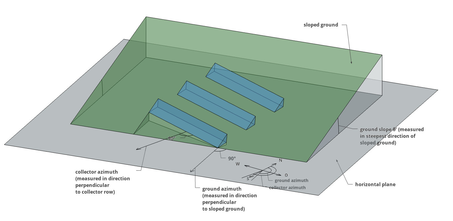
Figure 1: Overview of input quantities of the new shading algorithm.

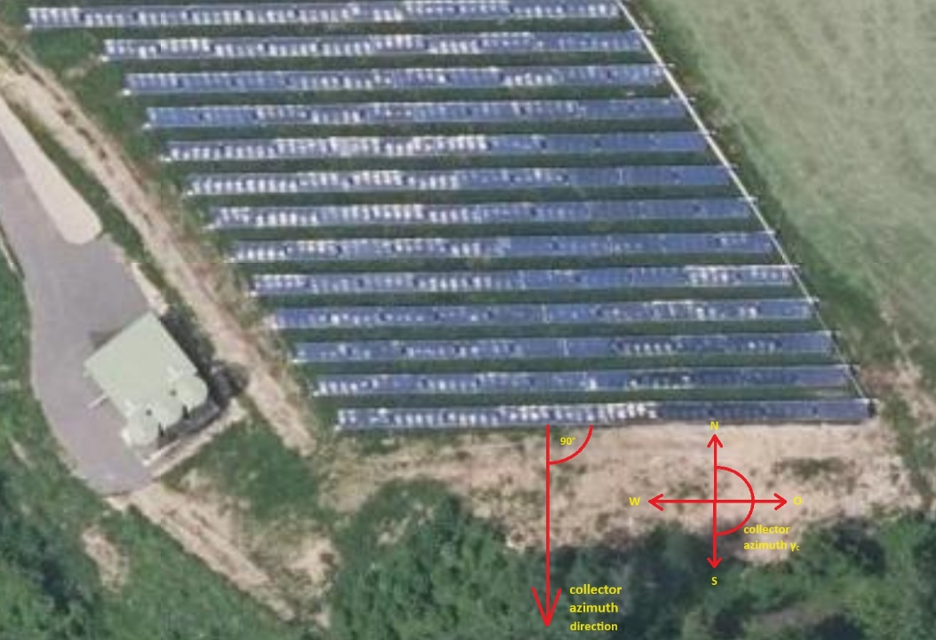
Figure 2: Collector azimuth angle, measured from satellite image. Image taken from the Styrian Digital Atlas [DigitalAtlas].

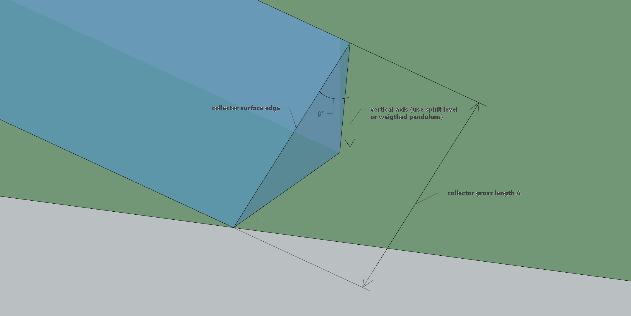
Figure 3: Collector tilt: \(\beta''\) is the absolute complementary tilt angle, i.e., the angle between collector surface edge and the plumb line (vertical axis).

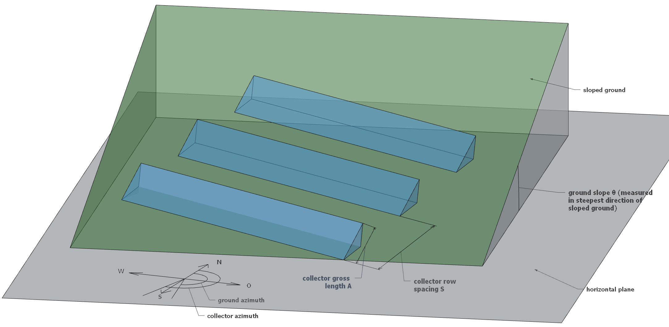
Figure 4: Measure collector gross length A and collector row spacing S.

Method

The procedure to evaluate the collector height for different collector and ground azimuths on sloped ground follows these main steps:

1. Calculation of ground slope in collector azimuth direction

2. Rotation of collector array area from horizontal mounting into obliquely mounted position on sloped ground

3. Definition of plane equation for collector surface

4. Calculation of collector tilt in collector azimuth direction

5. Calculation of virtual collector surface edge into collector azimuth direction

6. Shadow on an inclined pole

7. Calculation of shading fraction on collector surface

Calculation of ground slope in collector azimuth direction

The objective of this step is to calculate the actual ground slope \(\theta\) in the collector azimuth direction and the slope \(\epsilon\) perpendicular to the collector azimuth (line \(L''\) along the collector row in figure 5). Imagine the collector lies flat on the sloped ground (no tilt with respect to the sloped ground), rotated by an angle \(\gamma\) relative to the horizontal plane. By rotating the collector, the new slope in the collector azimuth direction \(\gamma_{c}\) can be determined (see Figure 5). This is necessary because initially, only the ground slope \(\theta'\) in the ground azimuth direction is known; remember that \(\theta\)‘ is measured in the steepest direction of the sloped ground, not in collector azimuth direction \(\gamma_{c}\). Additionally, the angle \(\epsilon\), normal to \(\theta\), is calculated. Calculating \(\theta\) and \(\epsilon\) requires only two inputs, namely \(\theta'\) (the ground slope) and \(\gamma\) (the azimuth difference between collector and ground). The calculations \(\theta\) (formula 2) and \(\epsilon\ \)(formula 3) can be found in Appendix A.1.

\[\gamma = \gamma_{c} - \gamma_{g} \qquad \qquad (\; 1\; )\]

\[\theta = \arctan\left( \cos\gamma \cdot \tan\theta^{'} \right) \qquad \qquad (\; 2 \; )\]

\[\epsilon = \arctan(\sin\gamma \cdot \tan\theta^{'}) \qquad \qquad ( \; 3 \; )\]

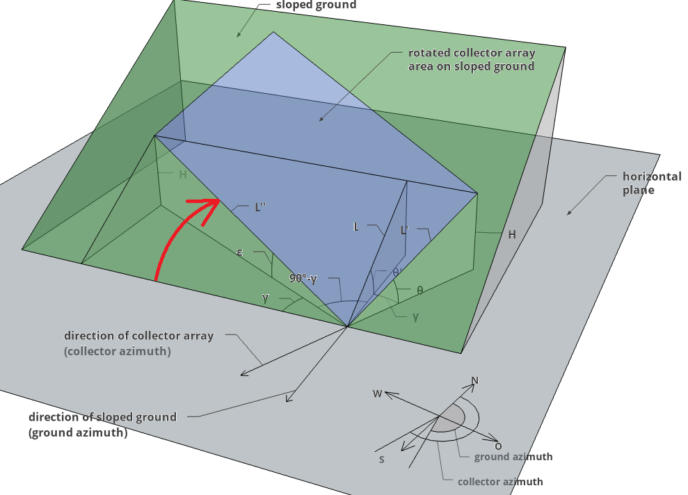
Figure 5: Rotation of collector array on sloped ground to evaluate the angles \(\theta\) and \(\epsilon\).

By knowing \(\theta\), \(\epsilon\), \(\gamma\)_c and the direction normal to \(\gamma\)_c, the rectangle representing the rotated collector on sloped ground is defined (blue area in Figure 5).

So far, only the sloped ground was considered and the direction angles that span the array on the sloped ground when obliquely mounted (see green area in Figure 5) are known. Up to this point, the collector tilt \(\beta'\) has not yet been considered; this is covered in the next step.

Rotation of collector into obliquely mounted position

This section addresses rotating the tilted collector from a horizontal mounted position to the obliquely mounted position on the sloped ground. Horizontal means that the tilt angle ε is assumed to be 0°. To determine the directions of the collector surface edges (see Figure 3 for the collector surface edge definition), we place the coordinate system in the horizontal plane (x-axis is green (only colored in negative direction), y-axis is red, z-axis is vertical), as illustrated in Figure 1. Note that the rotation around the azimuth difference angle \(\gamma\) in the horizontal plane is already done here. The unit vector \(\overrightarrow{r}\) indicates the direction of the collector surface edge if the collectors were mounted horizontally. It is placed in the z-y plane. We then rotate the vector \(\overrightarrow{r}\) by the angle \(\epsilon\) around the y-axis. The new direction \(\overrightarrow{r'}\) represents the collector surface edge after rotation (the red arrow in Figure 6 shows the rotation). \(\epsilon^{'}\) is the resulting angle between \(\overrightarrow{r}\) and \(\overrightarrow{r'}\). Note that in figure 6 the vector \(\overrightarrow{r}\) is not lying on the collector surface (blue plane). This is the case because r points along the collector surface edge before rotating the surface plane by the angle of \(\epsilon\) around the y-axis.

Figure 6: Rotation of unit vector \(\overrightarrow{r}\) \(\ \)around y-axis by angle \(\epsilon\)

\[\begin{split}\overrightarrow{r}\ = \begin{pmatrix} 0 \\ \cos(\theta + \delta) \\ \sin(\theta + \delta) \end{pmatrix} \qquad \qquad (\; 4 \; )\end{split}\]

The rotation matrix for a rotation around the y-axis is:

\[\begin{split}R_{y}(\epsilon)\ = \begin{pmatrix} \cos\epsilon & 0 & \sin\epsilon \\ 0 & 1 & 0 \\ -\sin\epsilon & 0 & \cos\epsilon \end{pmatrix} \qquad \qquad (\; 5 \; )\end{split}\]

The resulting unit vector \(\overrightarrow{r'}\) is then:

\[\begin{split}\overrightarrow{r'} = \ R_{y}(\epsilon) \cdot \overrightarrow{r} = \ \begin{pmatrix} \cos\epsilon & 0 & \sin\epsilon \\ 0 & 1 & 0 \\ - \sin\epsilon & 0 & \cos\epsilon \end{pmatrix} \cdot \begin{pmatrix} 0 \\ \cos(\theta + \delta) \\ \sin(\theta + \delta) \end{pmatrix} = \begin{pmatrix} \text{sin}\epsilon \cdot \text{sin}\left( \theta + \delta)\ \right.\ \\ \text{cos}\left( \theta + \delta)\ \right.\ \\ \text{cos}\epsilon \cdot \text{sin}(\theta + \delta) \end{pmatrix}\qquad(\;6\;)\end{split}\]

To determine \(\delta\), we use the input quantity \(\beta^{'}\), the absolute collector tilt (angle between collector surface edge and horizontal). Therefore, the z-component of \(\overrightarrow{r'}\) is the same as \(\sin{\left( \beta^{'} \right) = \cos(\beta''})\). Using equation 6, this yields an expression for \(\delta\):

\[sin\ \beta^{'} = cos\epsilon \cdot \sin\left( \theta + \delta) \right.\]

\[\delta = \arcsin\left( \frac{sin\ \beta^{'}}{cos\epsilon} \right) - \theta \; for \; (\theta + \delta) \; in \; interval\; [-90°, 90°] \qquad \qquad (\; 7 \; )\]

This yields the tilt angle of \(\overrightarrow{r}\) against the horizontal plane. It is denoted as χ.

\[\chi = \ \theta + \delta\]

\[\chi = \ \arcsin\left( \frac{sin\ \beta^{'}}{cos\epsilon} \right) \qquad \qquad (\;8\;)\]

Remember that \(\overrightarrow{r}\) would be the vector along the collector surface edge in collector azimuth direction, if \(\epsilon\) would be zero (this means in the case for \(\gamma_{g} = \gamma_{c}\) relation (7) would simplify to \(\chi = \ \beta^{'}\) ).

Definition of plane equation for collector surface

At this point all quantities that are needed to define the equation of plane for the collector surface are known. In order to define the plane, a reference point and two vectors which span the plane need to be known.

Two vectors we know are:

• The vector along the collector row (perpendicular to collector azimuth) on the sloped ground: \(\overrightarrow{b} = \begin{pmatrix} - \cos \epsilon \\ 0 \\ sin \epsilon \end{pmatrix}\ \)

• The vector along the collector surface: \(\overrightarrow{r'} = \begin{pmatrix} \sin \epsilon \cdot \sin \chi \\ \cos \chi \\ \cos \epsilon \cdot \sin \chi \end{pmatrix}\)

The equation of a plane is defined by

\[a \cdot \left( x - x_{0} \right) + \ b \cdot \left( y - y_{0} \right) + c \cdot \left( z - z_{0} \right) + d = 0 \qquad \qquad ( \; 9 \; )\]

The coordinates (\(x_{0},\ y_{0},\ z_{0})\)^T represent any vector that points from the origin to the plane. The surface plane is defined to be placed behind the first collector row with the calculated ground tilt in collector azimuth direction \(\theta\). Therefore the point P₁=(\(x_{0},\ y_{0},\ z_{0})\)^T\(= \ {(0,\ S \cdot \cos\theta,\ S \cdot \sin{\theta)}}^{T}\) lies on the plane. Remember that S is the collector row spacing. Figure 7 sketches the vectors \(\overrightarrow{b}\) and \(\overrightarrow{r'}\).

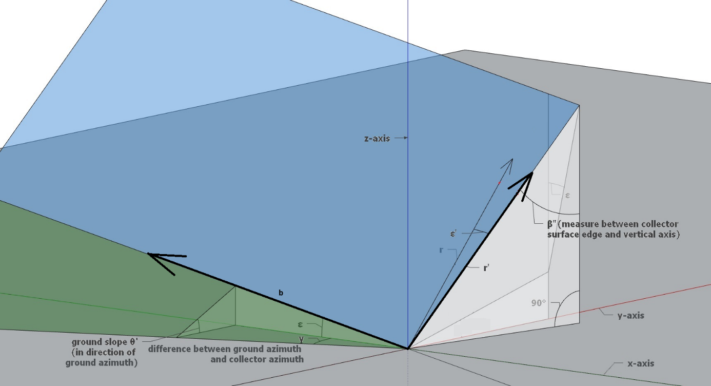
Figure 7: Definition of vectors b and r’

The coordinates (a, b, c)^T define the normal vector \(\overrightarrow{n}\ \)on the plane. Since two vectors, that both lie on the plane (\(\overrightarrow{r'}\) and \(\overrightarrow{b})\ \)are already known, \(\overrightarrow{n}\) can be defined by the vector product \(\overrightarrow{r'} \times \overrightarrow{b}\).

\[\begin{split}\overrightarrow{n} = \ \overrightarrow{r'} \times \overrightarrow{b} = \ \begin{pmatrix} \sin \epsilon \cdot \sin \chi \\ \cos \chi \\ \cos \epsilon \cdot \sin \chi \end{pmatrix}\ \times \begin{pmatrix} - \cos\epsilon \\ 0 \\ sin\epsilon \end{pmatrix} = \begin{pmatrix} \sin \epsilon \cdot \cos \chi \\ - \sin \chi \\ \cos \epsilon \cdot \cos \chi \end{pmatrix}\end{split}\]

The constant d is obtained by solving equation (9) for d using \(P_{1} = \left( x_{0},\ y_{0},\ z_{0} \right)^{T}\) and \(\overrightarrow{n} = (a,\ b,\ c)^{T}\)and setting \(x = y = z = 0\)

\[d = S \cdot (\cos \theta \sin \chi - \sin \theta \cos \epsilon \cos \chi)\]

Now the equation of plane for the collector surface as it is mounted on the sloped ground with different azimuths for collector and ground (\(\gamma_{c}\), \(\gamma_{g}\)) is entirely defined.

Calculation of collector tilt in collector azimuth direction

In order to evaluate the collector tilt angle of the collector in azimuth direction (angle β in figure 8), two points that lie on the y-axis (x=0) need to be found. Note that β projected on the horizontal has no x-coordinate, it lies on the y-axis. One point is already defined, the point P₁=(\(x_{0},\ y_{0},\ z_{0})\)^T\(= {(0,\ S \cdot \cos\theta,\ S \cdot \sin{\theta)}}^{T}\) from the section Definition of plane equation for collector surface. As second point any point which has a bigger y-coordinate than that of P₁ can be chosen, e.g. \(P_{2,y} = \ S \cdot \cos\theta + S \cdot \cos\chi\)

The corresponding z-coordinate of that specific point on the plane can be calculated by solving eq. (9) for z. This yields

\[P_{2,z} = \ \frac{\sin\chi\ \cdot P_{2,y} - \ S\ \cdot (\cos\theta\ sin\ \chi - \sin\theta\cos\epsilon\cos\chi)\ }{\text{cos}\epsilon \cdot \text{cos }\chi}\]

Knowing two points that lie on the plane with x-coordinate=0, the angle β can be calculated:

\[\beta = \tan^{- 1}\left( \frac{P_{2,z} - P_{1,z}}{P_{2,y} - P_{1,y}} \right) \qquad \qquad ( \; 10 \; )\]

Inserting the values for \(P_{2,z}\) and \(P_{2,y}\) the following equations remain:

\[P_{2,y} = y_{0} + S \cdot \cos \chi\]

\[P_{2,z} = z_{0} + \frac{S\ \cdot \sin\chi\ }{\text{cos}\epsilon}\]

\[\beta = \tan^{- 1}\left( \frac{\tan\chi\ }{\text{cos}\epsilon} \right)\]

Consequently, the unit vector \(\overrightarrow{a} = \begin{pmatrix} 0 \\ \cos\beta \\ \sin\beta \end{pmatrix}\) lies on the plane (origin not considered here)

Calculation of virtual collector surface edge in collector azimuth direction

In this step, we determine the length \(A^{'}\) of the virtual collector surface edge in collector azimuth direction. The virtual collector surface edge is oriented in the direction of \(\overrightarrow{a}\) with the yet unknown length \(A^{'}\) (see Figure 8). It is termed “virtual” because it represents the direction on the collector surface into collector azimuth direction, while the real collector surface edge points in the direction of \(\overrightarrow{r'}\). For this calculation, we use the dot-product formula \(\overrightarrow{a} \cdot \overrightarrow{b} = \left| \overrightarrow{a} \right||\overrightarrow{b}|\cos\alpha\). Let \(\epsilon^{'}\) be the angle between \(\overrightarrow{a}\ \)and \(\overrightarrow{r'}\) . Then:

\[\begin{split}\cos \epsilon^{'} = \overrightarrow{a} \cdot \overrightarrow{r^{'}} = \begin{pmatrix} 0 \\ \cos \beta \\ \sin \beta \end{pmatrix} \cdot \begin{pmatrix} \sin \epsilon \cdot \sin \chi \\ \cos \chi \\ \cos \epsilon \cdot \sin \chi \end{pmatrix}\end{split}\]

Solving this equation for \(\epsilon^{'}\) yields:

\[\epsilon^{'} = \arccos (\cos \beta \cdot \cos \chi + \cos \epsilon \cdot \sin \beta \cdot \sin \chi) \qquad \qquad (\; 11\; )\]

Given the collector gross length \(A\) as an input quantity and knowing \(\epsilon^{'}\) the virtual collector surface edge in collector azimuth direction, called A’ can be calculated.

\[A^{'} = \frac{A}{\cos \epsilon^{'}} \qquad \qquad (\; 12\; )\]

The projection of \(\overrightarrow{a}\) with length \(A'\) onto the z-axis gives the height of the virtual collector edge measured from the horizontal plane (see Figure 8):

\[H_{c} = A^{'} \cdot \sin \beta \qquad \qquad (\; 13 \; )\]

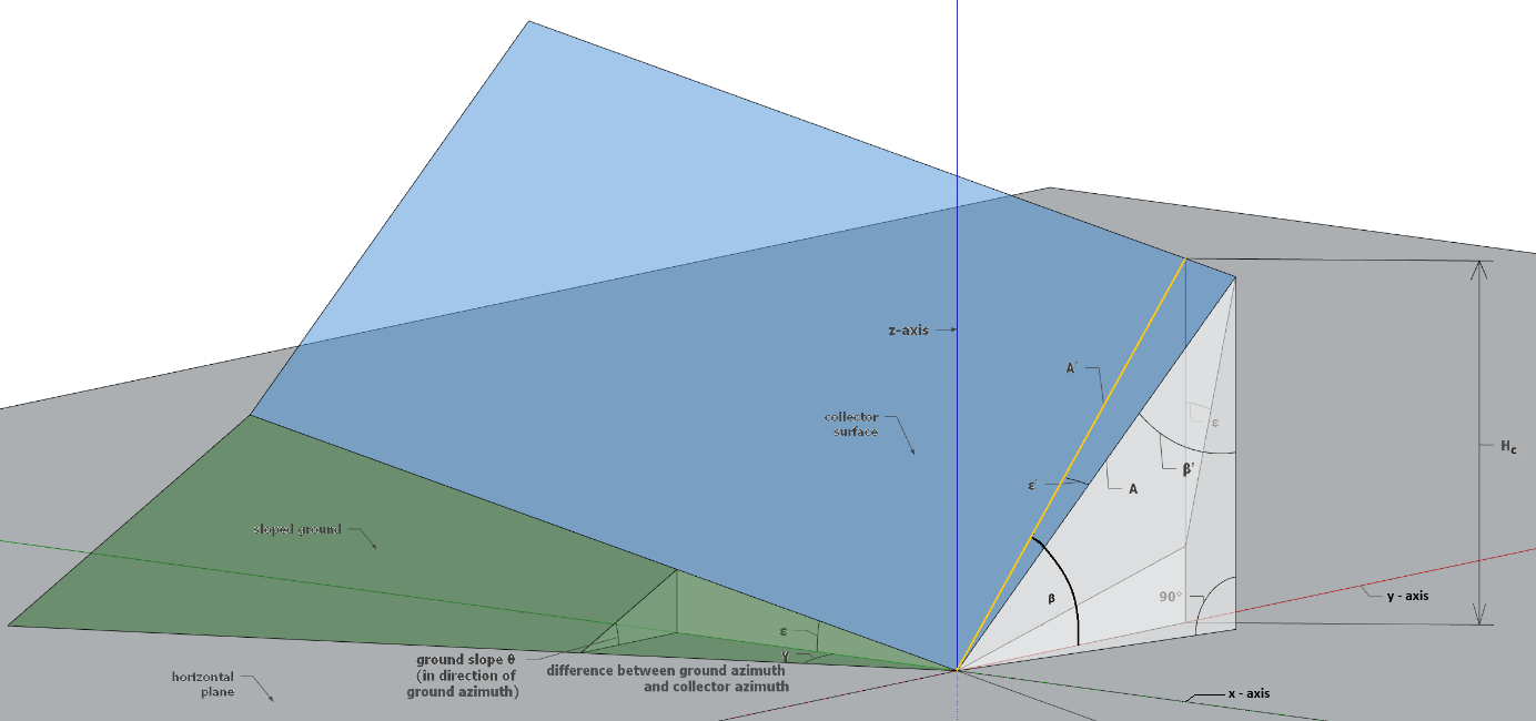
Figure 8: Visualization of virtual collector surface edge and collector tilt in collector azimuth direction β.

Shadow of an inclined pole

According to Bany and Appelbaum [BanyAppelbaum1987] the shadow components for x and y, named P_x and P_y, on an inclined pole OO’ (see Figure 9, taken from [BanyAppelbaum1987]) are:

\[P_{x} = \ \frac{A' \cdot {\sin\beta}{\cdot \sin\ \gamma_{S,rel}}}{\tan\alpha} \qquad \qquad (\; 14\; )\]

\[P_{y} = \left( \frac{A' \cdot {\sin\beta}{\cdot \cos\gamma_{S,rel}}}{\tan\alpha} \right) + A' \cdot \cos\beta \qquad \qquad (\; 15\; )\]

with \(\gamma_{S,rel} = \gamma_{s} - \gamma_{c}\) being the relative angle between sun azimuth \(\gamma_{S}\) and collector azimuth \(\gamma_{c}\), and with \(\alpha\) being the solar altitude angle.

Note that Bany and Appelbaum used the symbols A, \(\gamma_{s}\) and \(\mu\) instead of A’, \(\gamma_{S,rel}\), and β (see eq. A1 and A2 in [BanyAppelbaum1987]).

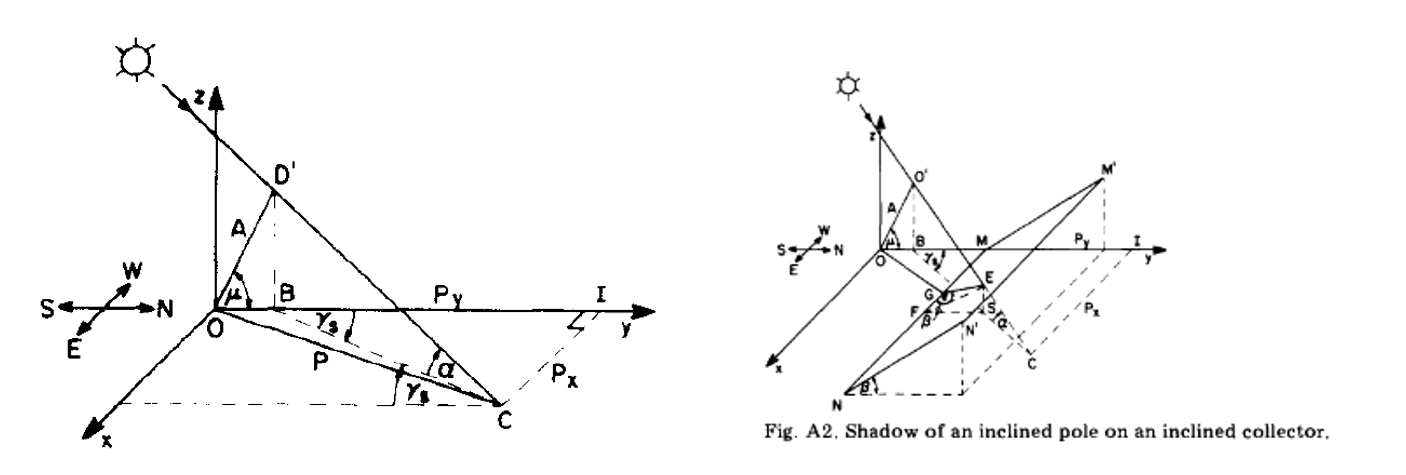
Figure 9: Shadow of an inclined pole, taken from Bany & Appelbaum [BanyAppelbaum1987]

The pole 0’C defines the tangent of the shadow behind the inclined pole 00’. The intersection-point of this tangent and the plane equation for the collector surface defined above is the point where the shadow hits the collector surface.

Calculation of tangent 0’C:

\[\begin{split}0^{'} = \begin{pmatrix} {0'}_{x} \\ {0'}_{y} \\ {0'}_{z} \end{pmatrix} = \begin{pmatrix} 0 \\ A' \cdot \cos\beta \\ A' \cdot \sin\beta \end{pmatrix}, \qquad \qquad Point\; C = \begin{pmatrix} C_{x} \\ C_{y} \\ C_{z} \end{pmatrix} = \begin{pmatrix} P_{x} \\ P_{y} \\ 0 \end{pmatrix}\end{split}\]

\[\begin{split}T: \qquad \qquad \begin{pmatrix} x \\ y \\ z \end{pmatrix} = \begin{pmatrix} {0'}_{x} \\ {0'}_{y} \\ {0'}_{z} \end{pmatrix} + t \cdot \begin{pmatrix} C_{x} - {0^{'}}_{x} \\ C_{y} - {0^{'}}_{y} \\ C_{z} - {0^{'}}_{z} \end{pmatrix} = \begin{pmatrix} 0 \\ A^{'} \cdot \cos\beta \\ A^{'} \cdot \sin\beta \end{pmatrix} + t \cdot \begin{pmatrix} P_{x} - 0 \\ P _{y} - A' \cdot \cos\beta \\ 0 - A' \cdot \sin\beta \end{pmatrix} \\ = A^{'}\begin{pmatrix} 0 \\ \cos\beta \\ \sin\beta \end{pmatrix} + t \cdot \frac{A^{'} \cdot \sin\beta}{\tan\alpha}\begin{pmatrix} \sin\gamma_{S,rel} \\ \cos\gamma_{S,rel} \\ - \tan\alpha \end{pmatrix} \qquad \qquad \qquad (\; 16\; ) \qquad \qquad\end{split}\]

Calculation of shading fraction on collector surface

To get to the final result of shading fraction on the collector the shading point E on the collector needs to be computed. This is done by calculating the intersection point of the tangent equation (16) and the plane equation of the collector surface. Secondly the geometric point on the bottom of the collector surface, named F, needs to be evaluated. The absolute shading is then the pole FE. The shading fraction is the relative distance [0, 1].

The parameter t needs to be solved by equating the tangent equation T and equation (9).

It yields:

\[t = \frac{a \cdot {0^{'}}_{x} + b \cdot {0^{'}}_{y} + c \cdot {0^{'}}_{z} + d}{a \cdot {0^{'}}_{x} - a \cdot C_{x} + b \cdot {0^{'}}_{y} - b \cdot C_{y} + c \cdot {0^{'}}_{z} - c \cdot C_{z}} = \frac{b \cdot A' \cdot \cos\beta + c \cdot A' \cdot \sin\beta + d} {a \cdot P_{x} + b \cdot A' \cdot \cos\beta - b \cdot P_{y} + c \cdot A' \cdot \sin\beta}\]

Which can be simplified to:

\[t = \frac{\tan\alpha}{A^{'} \cdot \sin\beta} \cdot \frac{\sin \chi \cdot \left( S\cos\theta - A^{'} \cdot \cos\beta \right) + \cos \epsilon \cdot \cos\chi \cdot \left( A^{'} \cdot \sin\beta - S \cdot \sin\theta \right)}{\left( \sin \chi \cdot \cos \gamma_{s,rel} - \sin \epsilon \cdot \cos \chi \cdot \sin \gamma_{s,rel}+\tan \alpha \cdot \cos \epsilon \cdot \cos \chi \right)}\]

Resulting in the following equation for the point E

\[\begin{split}E = A^{'}\begin{pmatrix} 0 \\ \cos\beta \\ \sin\beta \end{pmatrix} + t_{E} \cdot \begin{pmatrix} \sin\gamma_{s,rel} \\ \cos\gamma_{s,rel} \\ - \tan\alpha \end{pmatrix}\end{split}\]

with the adjusted factor \(t_{E}\) and using \(D\) and \(H\) for the distance between the collectors (back to front) and H as the height difference between collector top and the bottom of the collector on the next row.

\[t_E=\frac{\sin \chi \cdot D+\cos \epsilon \cdot \cos \chi \cdot H}{\left(\sin \chi \cdot \cos \gamma_{s, \text { rel }}-\sin \epsilon \cdot \cos \chi \cdot \sin \gamma_{s, \text { rel }}+\tan \alpha \cdot \cos \epsilon \cdot \cos \chi\right)}\]

\[D = S\cos\theta - A^{'} \cdot \cos\beta \qquad \qquad (\; 17\; )\]

\[H = \ H_{c} - S \cdot \sin \theta = A^{'} \cdot \sin\beta - S \cdot \sin\theta \qquad \qquad (\; 18\; )\]

Note that the equation greatly simplifies in case of no ground tilt perpendicular to the collector surface \(\epsilon = 0\).

\[t_{E}(\epsilon = 0) = \frac{\sin \chi \cdot D + \cos\chi \cdot H}{\sin \chi \cdot \cos \gamma_{s,rel} + \cos \chi\cdot \tan \alpha} \qquad \qquad (\; 19\; )\]

In order to evaluate the shading fraction on the collector surface, the geometric point on the bottom of the collector surface, named F, needs to be evaluated. With the information now available about the geometry and since the intersection point E is known, the point F can also be easily defined. For a better understanding look at Figure 9. Note that figure 9 taken from Bany and Appelbaum [BanyAppelbaum1987] covers only the case of no ground slope (\(\theta = 0{^\circ}\)). However, for a better understanding of the geometry it should also help.

The x-component of F is the same as the x component of E, as we want to know the lowest point of the collector at the same row-position (x-value) where the sun beam intersects with the collector. Hence, \(F_x = E_x\).

For the y-component (along the collector azimuth), we know that the lowest point of the collectors is positioned at \(F_{y}= S \cos \theta\) which is essentially the row distance between the first collector row and the next collector row.

For the z-direction, we know that the second collector row is higher than the first collector row by \(S \sin \theta\) due to the ground tilt. However, we need to subtract \(\tan \epsilon \cdot E_x\) in order to take into account that the ground is tilted perpendicular to the collector azimuth, which decreases the height in x direction (note that \(\epsilon\) is defined in negative x-axis direction (see e.g. Figure 6 or 7).

Finally, F can be written as:

\[\begin{split}F = \begin{pmatrix} E_{x} \\ S\ \cdot \cos\theta \\ S\ \cdot \sin\theta - \tan \epsilon \cdot E_x \end{pmatrix}\end{split}\]

In the case of E_y > F_y the pole FE is the absolute shading fraction on the collector surface:

\[FE = \ \sqrt{\left( E_{x} - F_{x} \right)^{2} + \left( E_{y} - F_{y} \right)^{2} + \left( E_{z} - F_{z} \right)^{2}} = \sqrt{\left( E_{y} - S\ \cdot \cos\theta \right)^{2} + \left( E_{z} - S\ \cdot \sin\theta + \tan\epsilon \cdot E_{x}) \right)^{2}}\]

Which can be rewritten as:

\[FE = \sqrt{{dy}^{2} + {dz}^{2}} \qquad \qquad (\; 20\; )\]

\[dy = t_E \cdot \cos \gamma_{s,rel} - D\]

\[dz = H - t_E \left( \tan \alpha - \tan \epsilon \cdot \sin \gamma_{s,rel} \right)\]

The relative shading fraction is defined as

\[h_{s} = \frac{FE}{A'}\]

In the case of \(E_y < F_y\) the absolute and therefore also the relative shading fraction is \(< 0\). By definition the shading fraction for that case is defined to be 0, since the collector rows then will not be shaded. In the case that the shadow pole intersects with the surface plane at a larger y-coordinate than at the top of the collector surface (in case of \(E_y > S \cdot \cos \theta + A' \cdot \cos \beta\)), the shading fraction is set to 1. This is done because for that case the collector surface is shaded entirely.

\[\begin{split}h_{s} = \left\{ \begin{matrix} 0 & if\ \left( t_{E} \cdot \cos\gamma_{S,rel} - D \right) < 0 \\ \frac{FE}{A^{'}} & if\ 0 \le \left( t_{E} \cdot \cos\gamma_{S,rel} - D \right) \le A' \cdot \cos \beta \\ 1 & if\ \left( t_{E} \cdot \cos\gamma_{S,rel} - D \right) > A' \cdot \cos \beta \end{matrix} \right. \qquad \qquad (\; 21\; )\end{split}\]

This is the final result for evaluation of the internal shading fraction for the case of different collector- and ground azimuths (\(\gamma_{g} \neq \gamma_{c}\)) on sloped ground.

Diffuse Masking

For collectors within a collector field, the view obstruction of the front collector row reduces the incident diffuse radiation from the sky. This effect is called diffuse masking and also alters reflection patterns. These phenomena are not addressed in ISO 24194.

Diffuse masking is more pronounced for narrow row spacing and steep collector tilt angles, and can substantially reduce the diffuse irradiance in the plane of the array. For reference, measurements showed a reduction to 89% on average, relative to the top of the collector (=100%), for a collector field with 3.5 m row spacing, 45° tilt angle, and 1.67 relative row spacing [Tschopp2022].

Not taking diffuse masking into account in Power Check overestimates the collector field’s \(G_d\) and \(G_{hem}\), resulting in a higher estimated power output and shifting the measured-estimated power ratio unfavorably compared to the true performance.

To account for diffuse masking for narrow row spacings and steep collector tilts, a radiation correction model should be used (e.g., [Tschopp2022] or the Passias model available in pvlib), or a slightly higher safety factor.

Note

Diffuse masking is not yet implemented in SunPeek. Future versions may include automatic diffuse masking corrections based on array geometry.

Literature

[Anderson2020]

Anderson, K. & Mikofski, M. Slope-Aware Backtracking for Single-Axis Trackers (2020). NREL/TP–5K00-76626, https://doi.org/10.2172/1660126.

[BanyAppelbaum1987] (1,2,3,4,5,6,7,8)

J. Bany and J. Appelbaum, “The effect of shading on the design of a field of solar collectors,” Solar Cells, vol. 20, no. 3, pp. 201-228, 1987, doi:10.1016/0379-6787(87)90029-9.

[AppelbaumBany1979] (1,2)

J. Appelbaum and J. Bany, “Shadow effect of adjacent solar collectors in large scale systems,” Solar Energy, vol. 23, no. 6, pp. 497-507, 1979, doi:10.1016/0038-092X(79)90073-2.

[Tschopp2022] (1,2)

D. Tschopp, A. R. Jensen, J. Dragsted, P. Ohnewein, and S. Furbo, “Measurement and modeling of diffuse irradiance masking on tilted planes for solar engineering applications,” Sol. Energy, vol. 231, pp. 365-378, 2022, doi:10.1016/j.solener.2021.10.083.

[DigitalAtlas]

“Digitaler Atlas Steiermark :: KartenPortal.” Accessed: Jun. 18, 2024. [Online]. Available: https://gis.stmk.gv.at/wgportal/atlasmobile

Appendix

Calculation of ground slope in collector azimuth direction

For a triangle with sides \(a\), \(b\), \(c\), and with opposite respective angles \(\alpha\), \(\beta\) and \(\gamma\) (see Figure 1), the law of cosines states: \(c^{2} = a^{2} + b^{2} - 2ab\cos\gamma\)

For our problem, this yields:

\[H^{2} = L^{2} + {(L\cos{\theta')}}^{2} - 2L^{2}\cos^{2}\theta' \qquad \qquad ( \; A.1 \; )\]

Note that in Figure 5, the length \(L\cos\theta\)‘ is defined as \(T\). \(L\) and \(H\) can be expressed as:

\[L = L^{'}\ \frac{\cos\theta}{\cos{\theta'}}\ \cos\gamma\]

\[H = L^{'}sin(\theta)\]

Putting expressions for \(L\) and \(H\) in equation A.1 gives:

\[L^{'2}{\sin}^{2}(\theta) = L^{'2} {\cos}^{2}(\theta){\cos}^{2}\gamma\ \left\lbrack \frac{1}{\cos^{2}\theta^{'}} - 1 \right\rbrack \qquad \qquad ( \; A.2 \; )\]

This can be solved for \(\theta\):

\[\theta = \arctan\left( \cos\gamma \cdot \tan\theta^{'} \right) \qquad \qquad ( \; A.3 \; )\]

\(\epsilon\) is the slope in direction normal to \(\gamma_c\) (see Figure 5). It can be evaluated in the same way as \(\theta\) with the only difference that the angle between the two directions now is \((90{^\circ} - \gamma)\). Therefore, the calculation yields:

\[\epsilon = \arctan\left( \cos{(90{^\circ} - \ \gamma)} \cdot \tan{\theta'} \right) = \arctan(\sin\gamma \cdot \tan{\theta'}) \qquad \qquad ( \; A.4 \; )\]

Example Plots

Here are a few plots to illustrate numeric results for the internal shading fraction of the new Sloped Ground algorithm for selected choices of ground and collector field azimuth, and tilt angles.

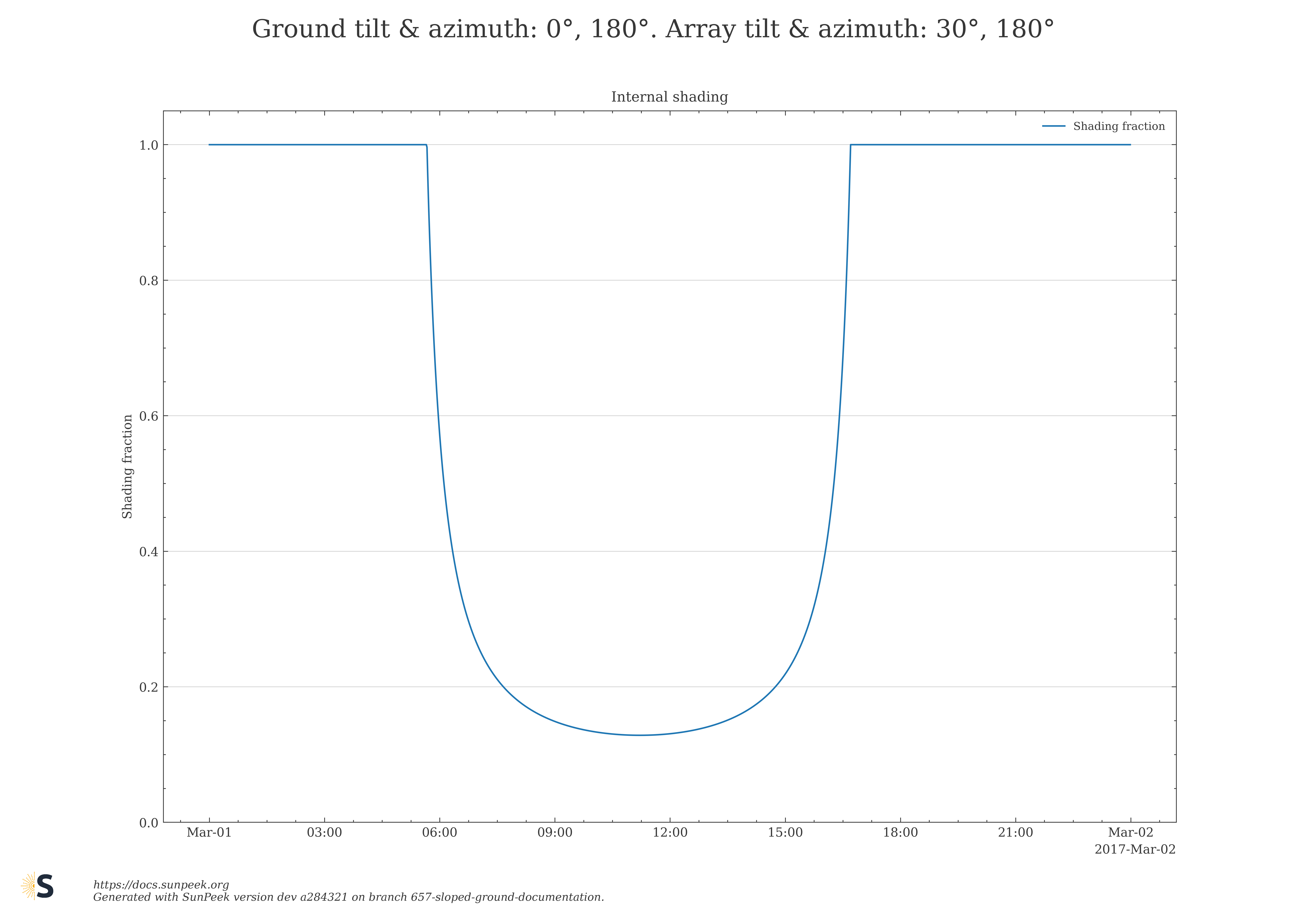
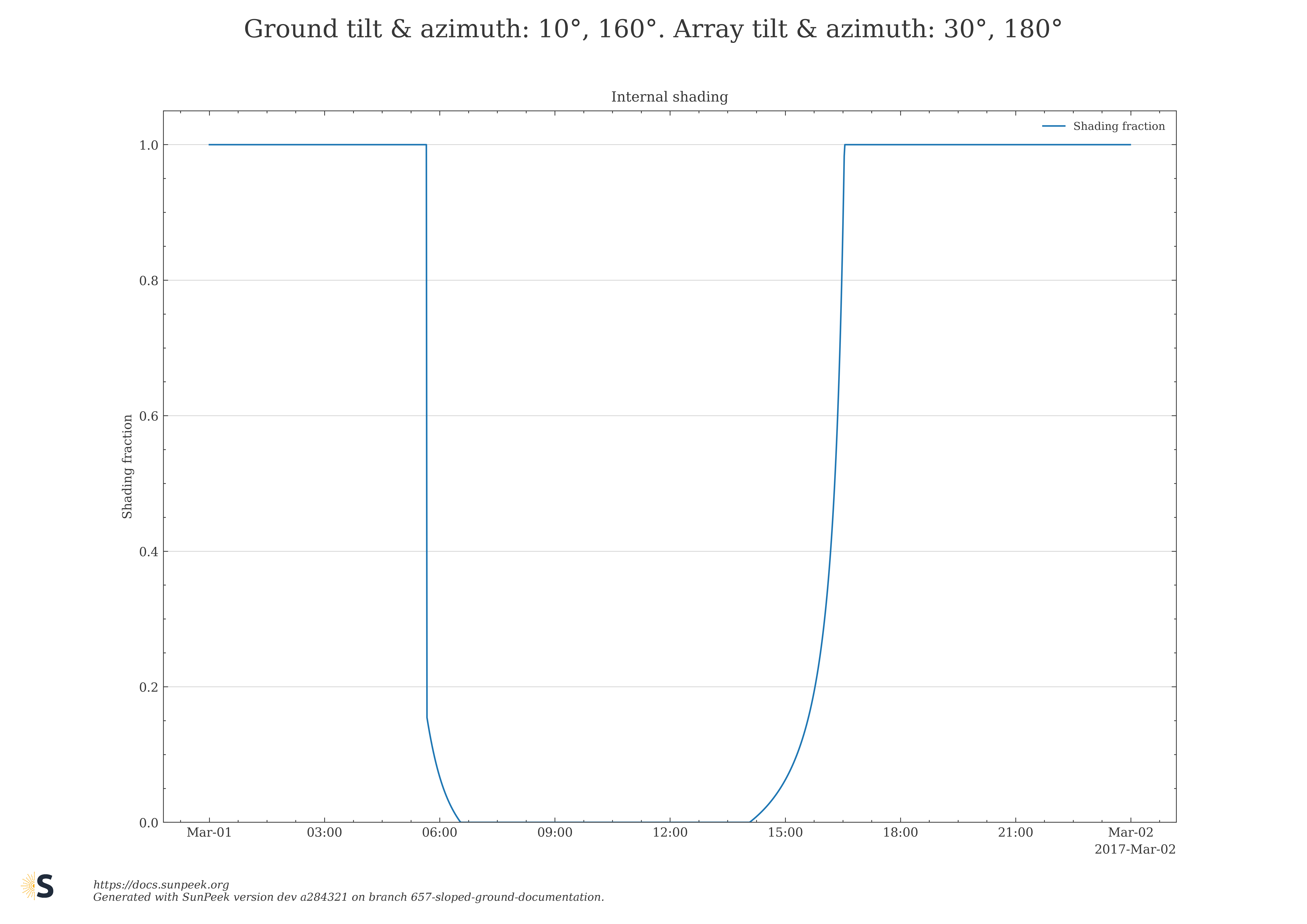
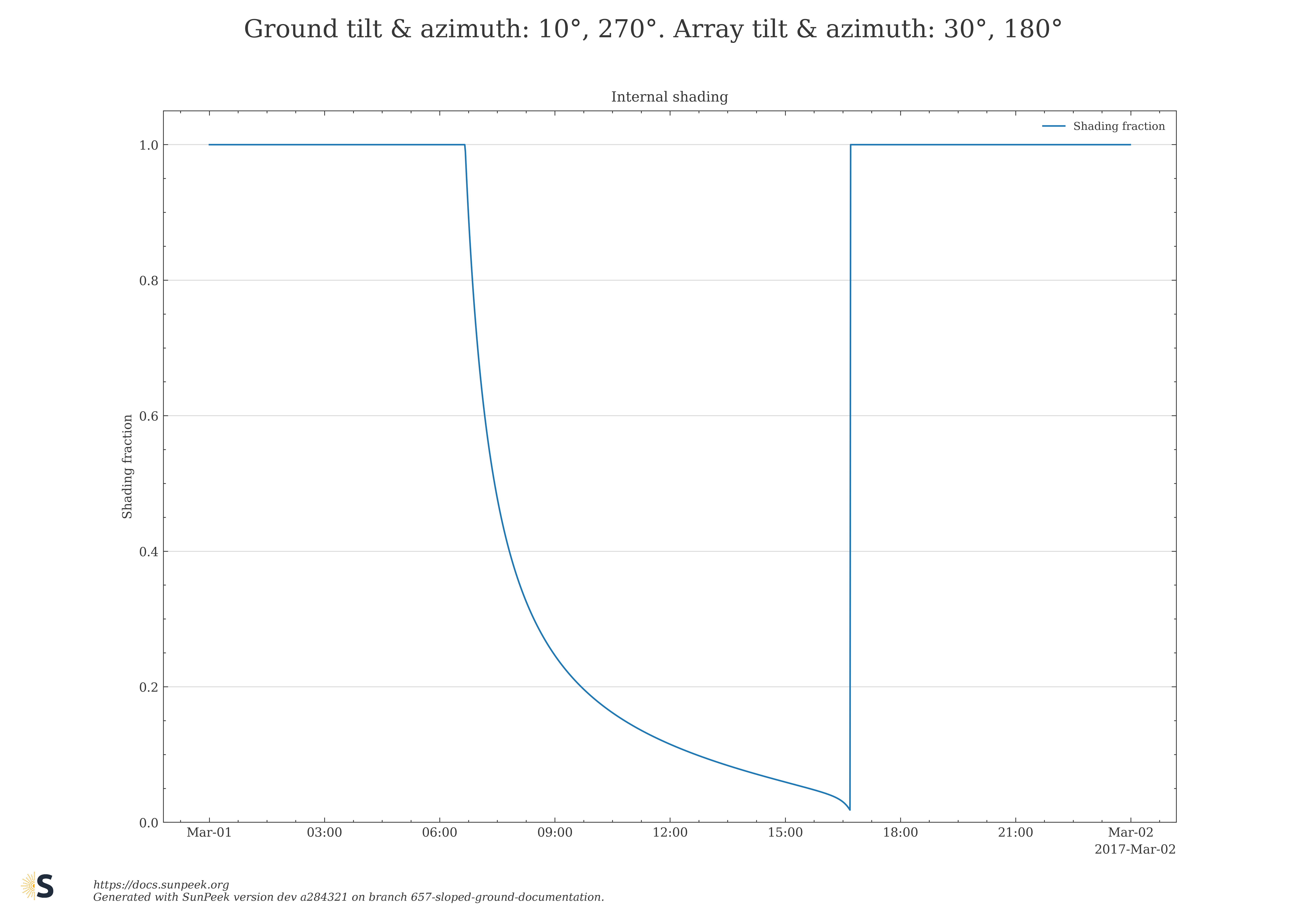
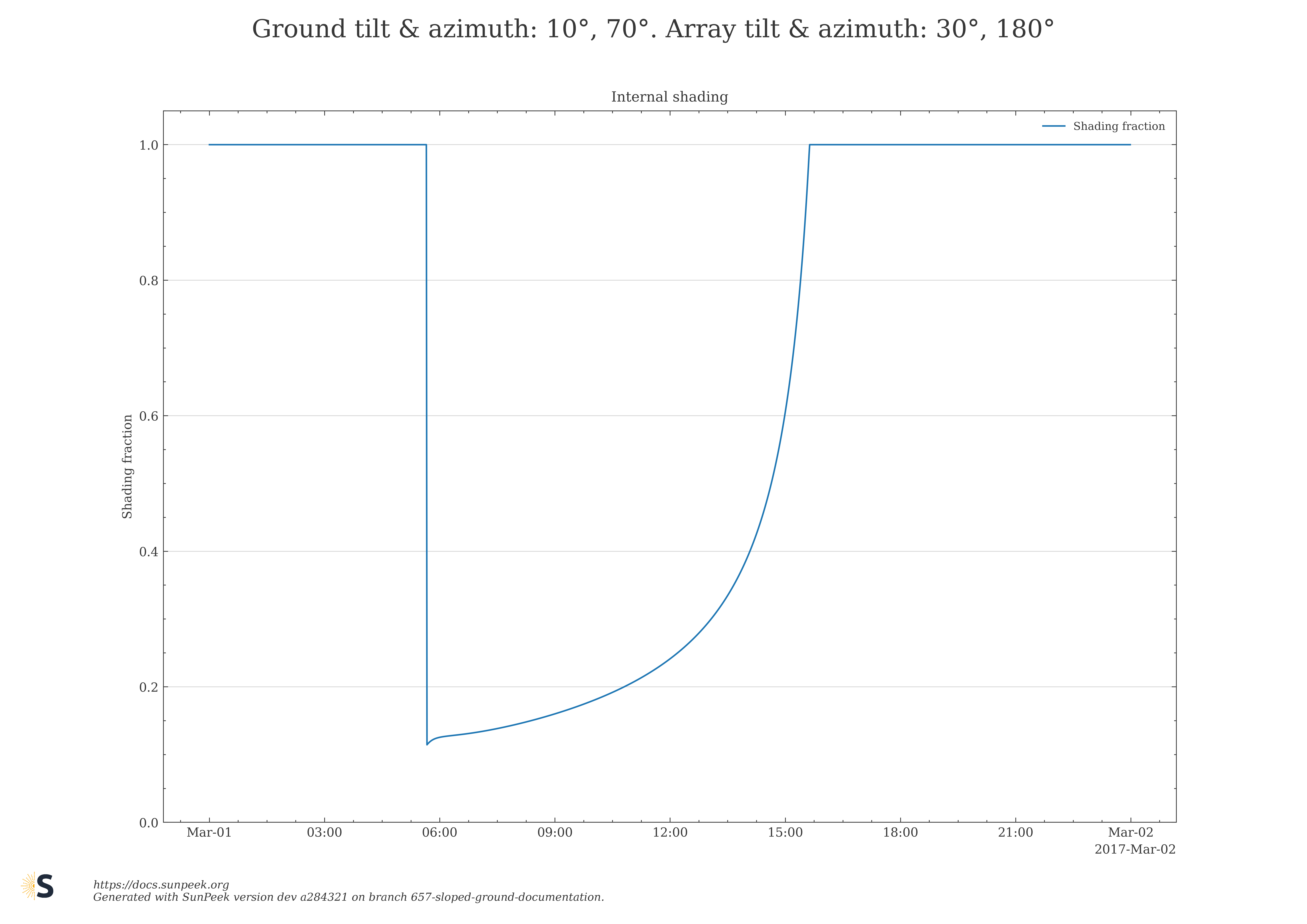
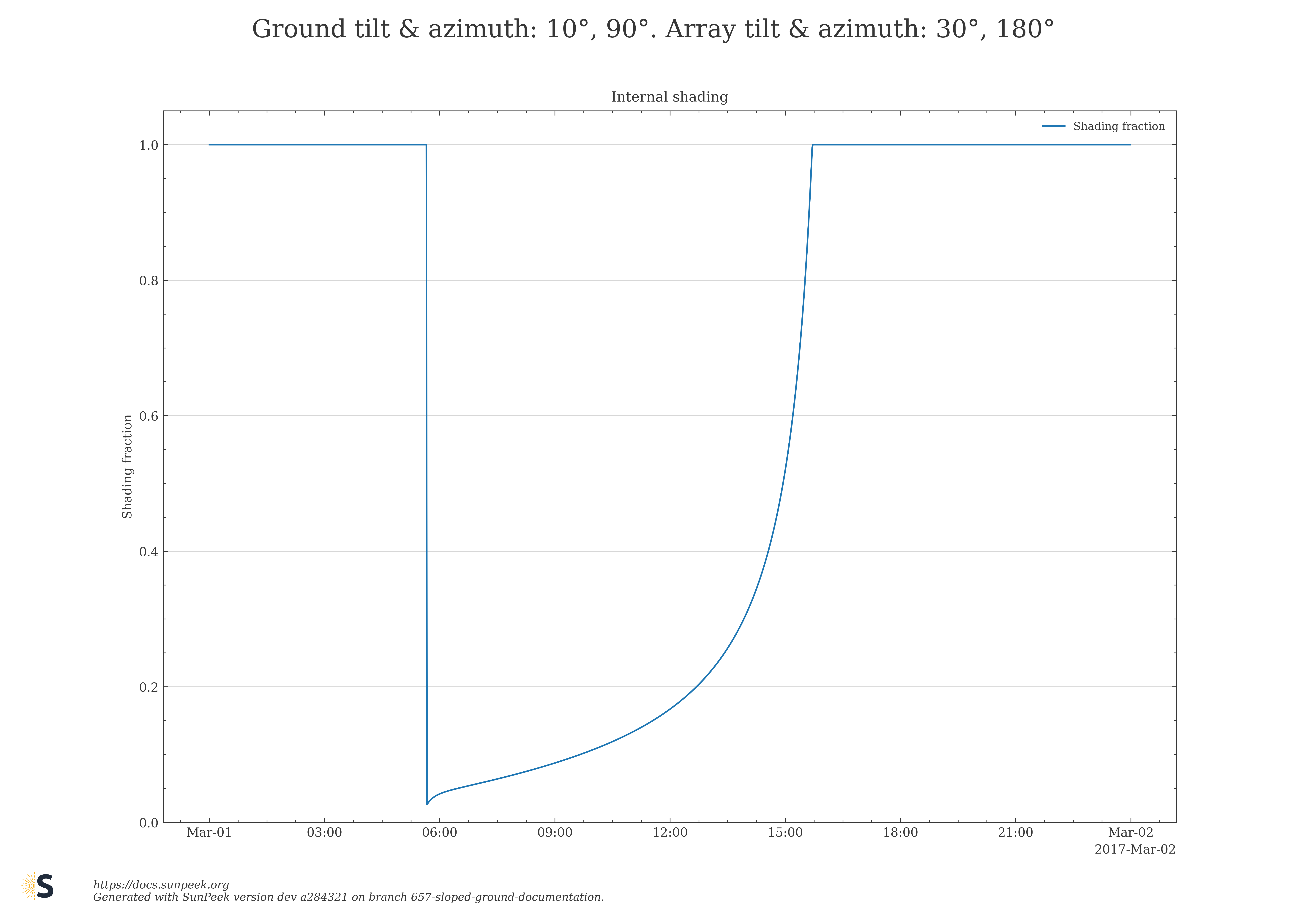
Figure 10: Numeric results for the internal shading fraction obtained with the Sloped Ground algorithm for selected choices of ground and collector field azimuth, and tilt angles.

Comparison with classical Bany Appelbaum

In this section, a few plots shall highlight the differences in output and compare the classical Bany Appelbaum with the new Sloped Ground algorithm. The new algorithm extends Bany Appelbaum by supporting different azimuth angles (of ground and collector field).

Figure 11 shows the shading fraction computed with both algorithms (classical Bany Appelbaum, new Sloped Ground algorithm), for the special case where ground and collector field face in the same azimuth direction (azimuth_ground = azimuth_collector_field). The comparison is done for a ground tilt of 0° (completely flat ground) and 6°. Such a ground tilt (but in same azimuth direction) is also supported by the classical Bany Appelbaum. The two curves overlap showing that the numeric results of the two algorithms are, in this special case, identical.

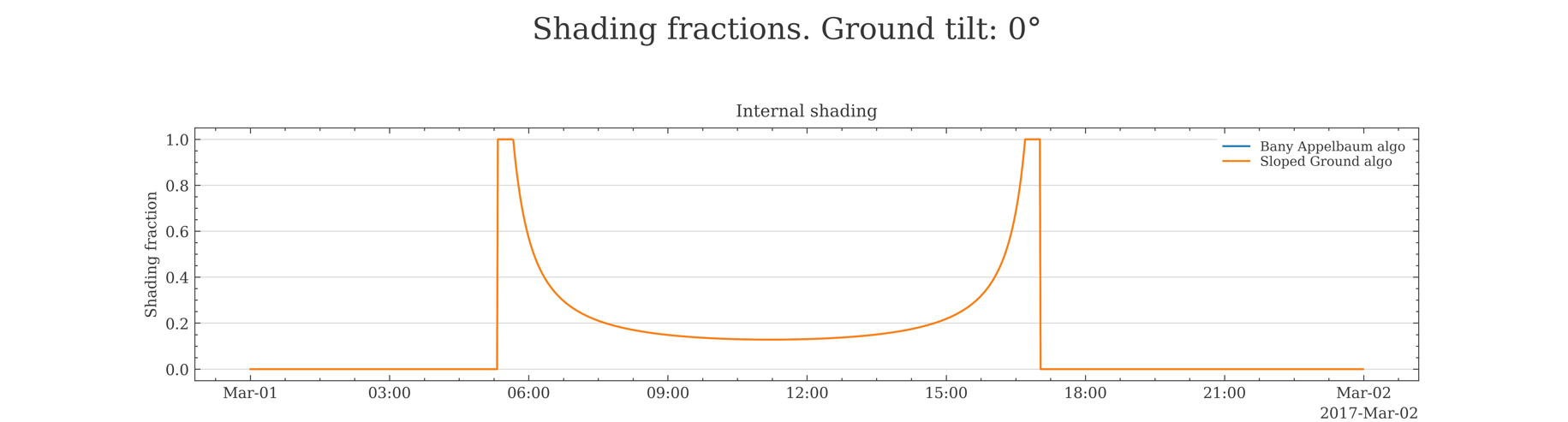
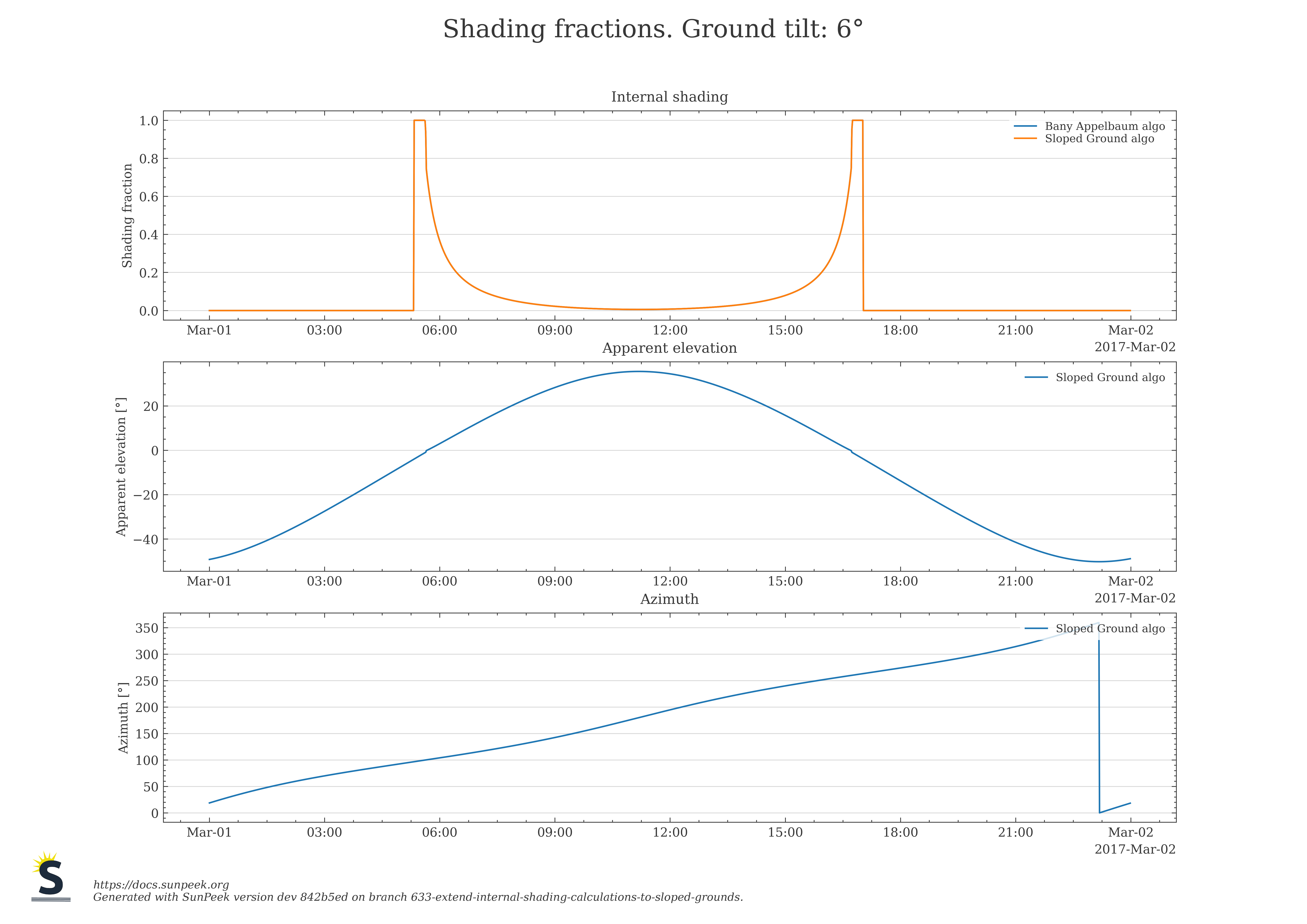
Figure 11: Shading fraction computed with classical Bany Appelbaum algorithm and new Sloped Ground algorithm for horizontal ground (0°, left) and for sloped ground (6°, right)

Next, results for Bany Appelbaum and the new Sloped Ground algorithm are shown in Figure 12, where collector azimuth and ground azimuth slightly deviate from each other. The plots on the left side are shown for flat ground, the plots on the right show results for a tilted ground of 6°. It is observable that the two algorithms give deviating results for the shading fraction as soon as the azimuth is not the same any more, but the results are identical in case of equal azimuth for Bany Appelbaum and the new sloped ground algorithm, which can be seen as a proof that the results match the expectations.

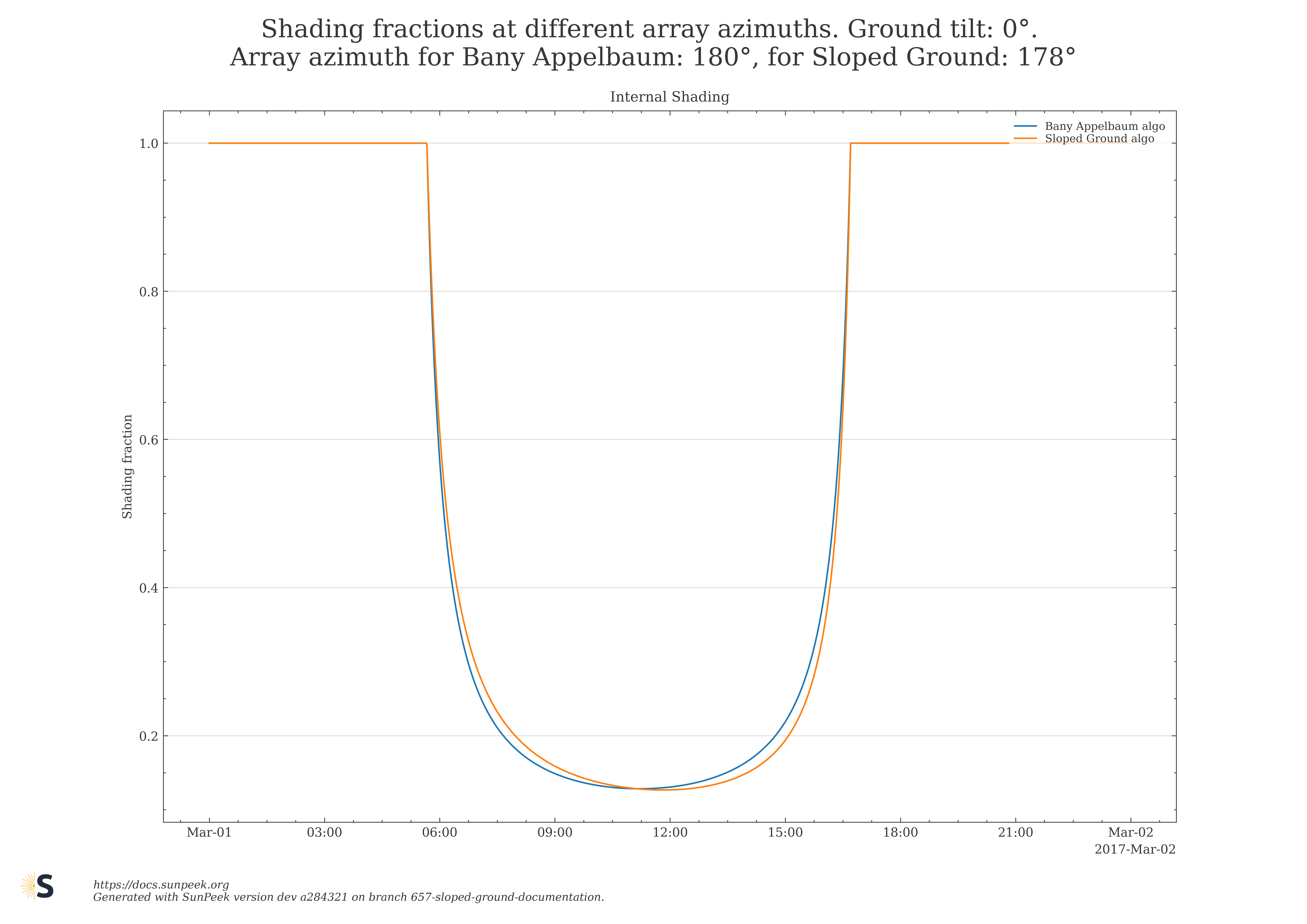
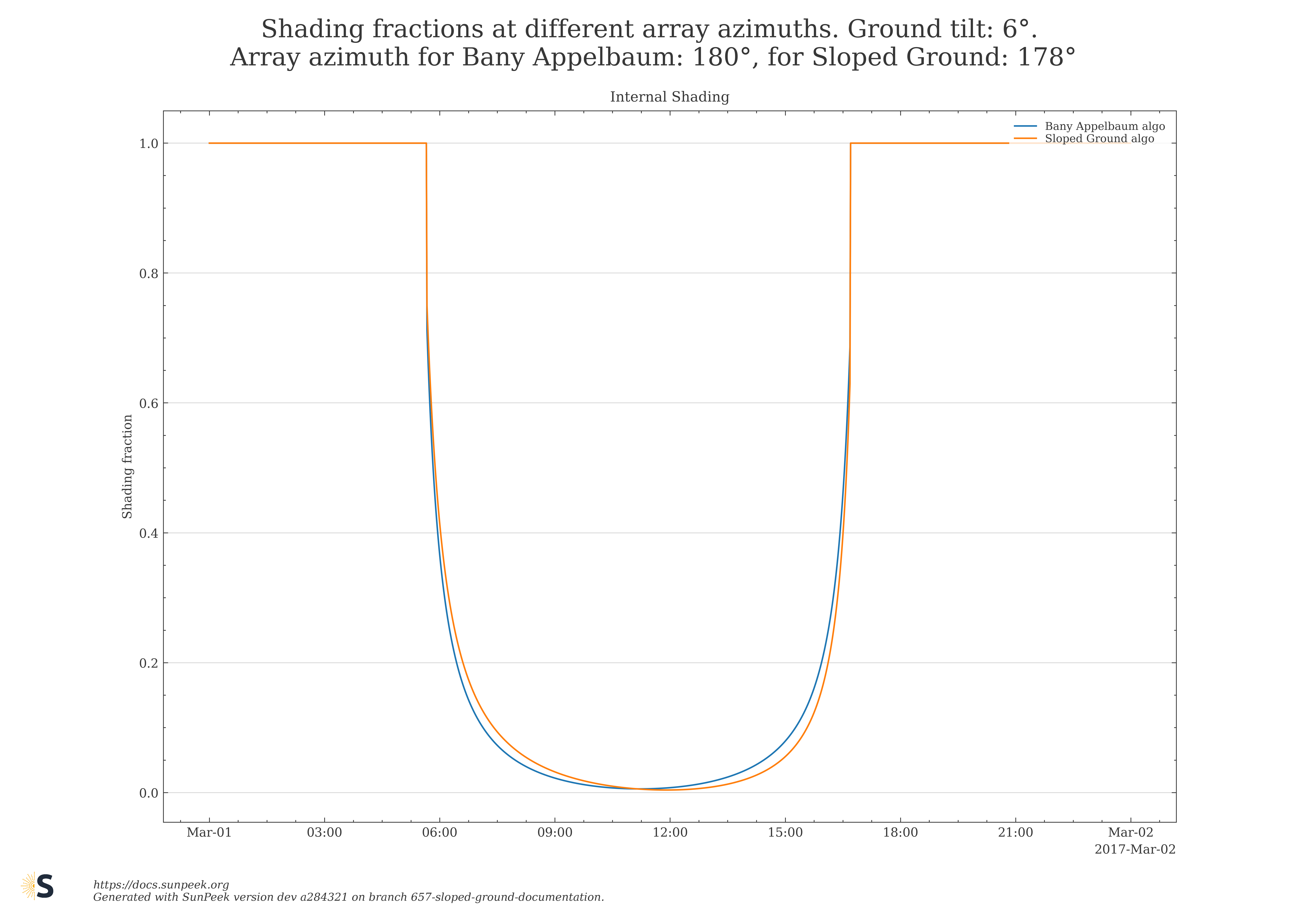
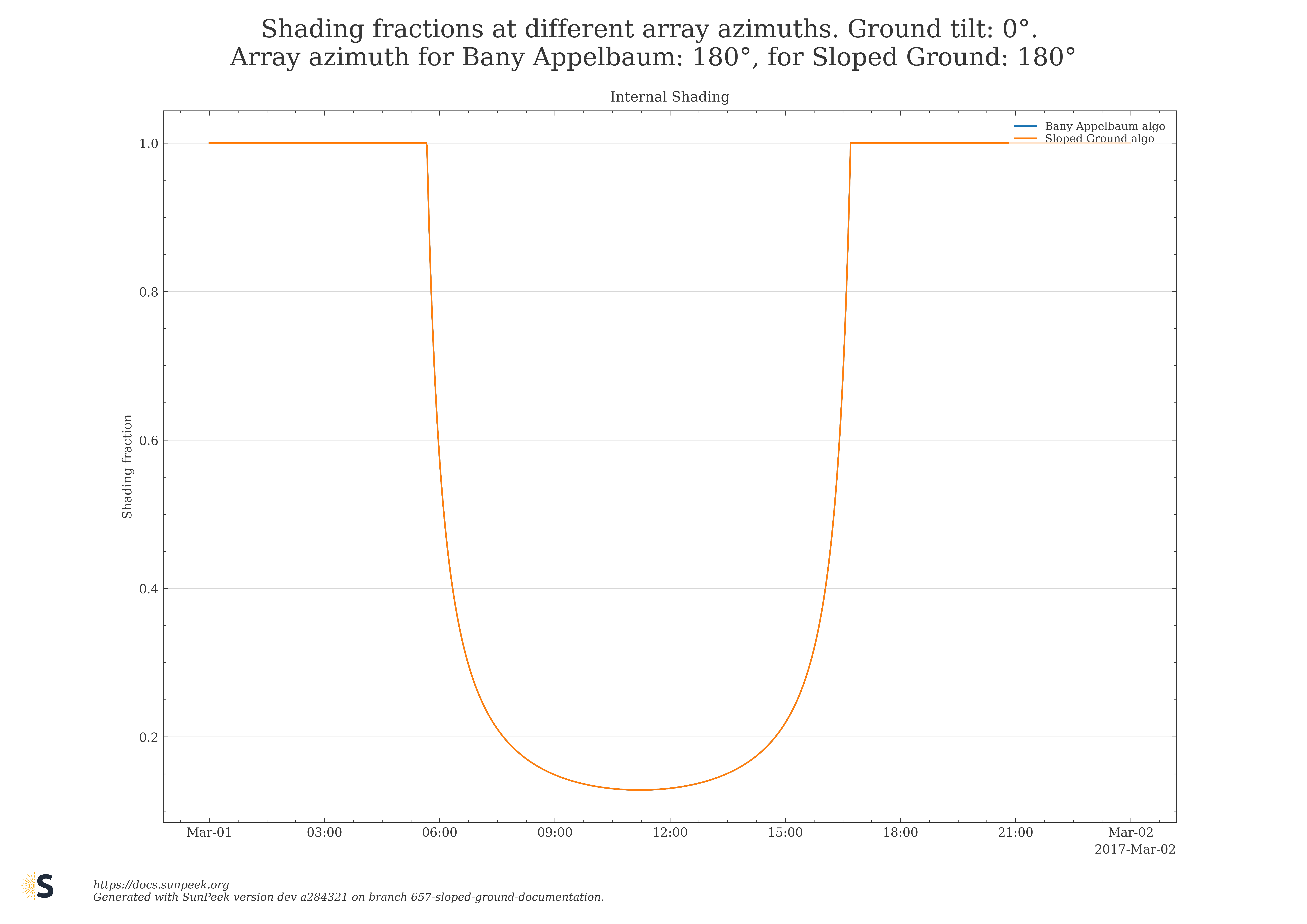
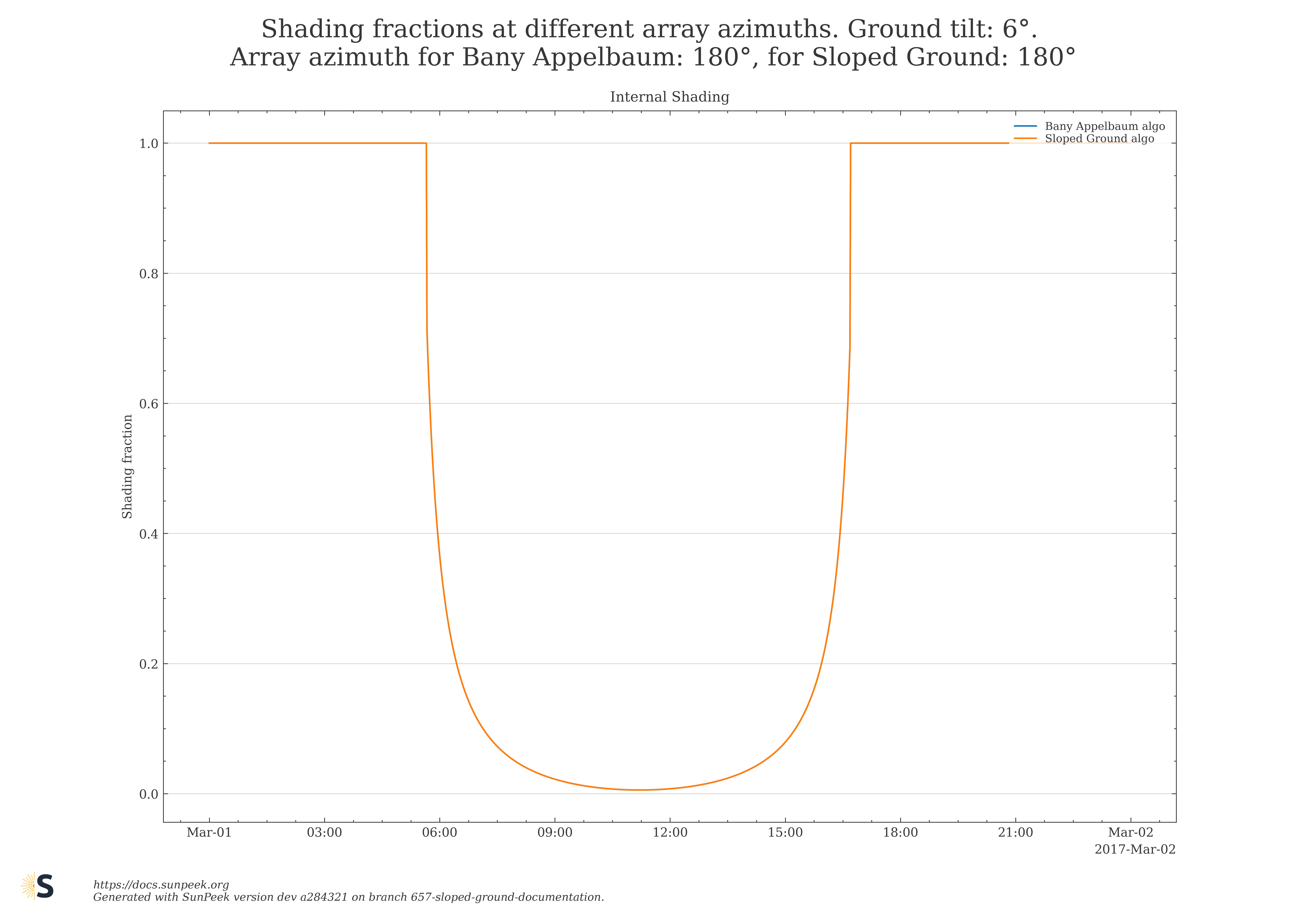
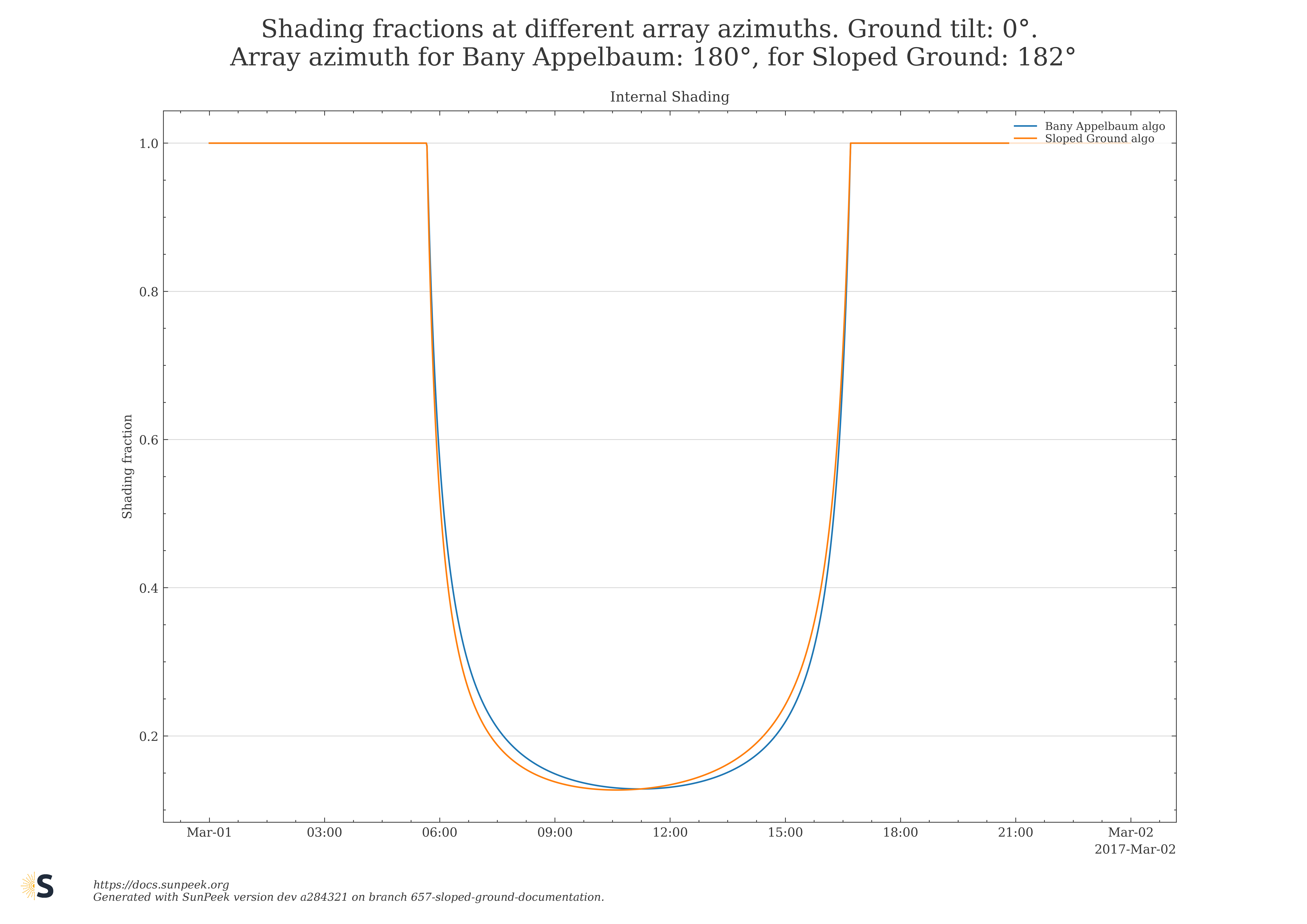
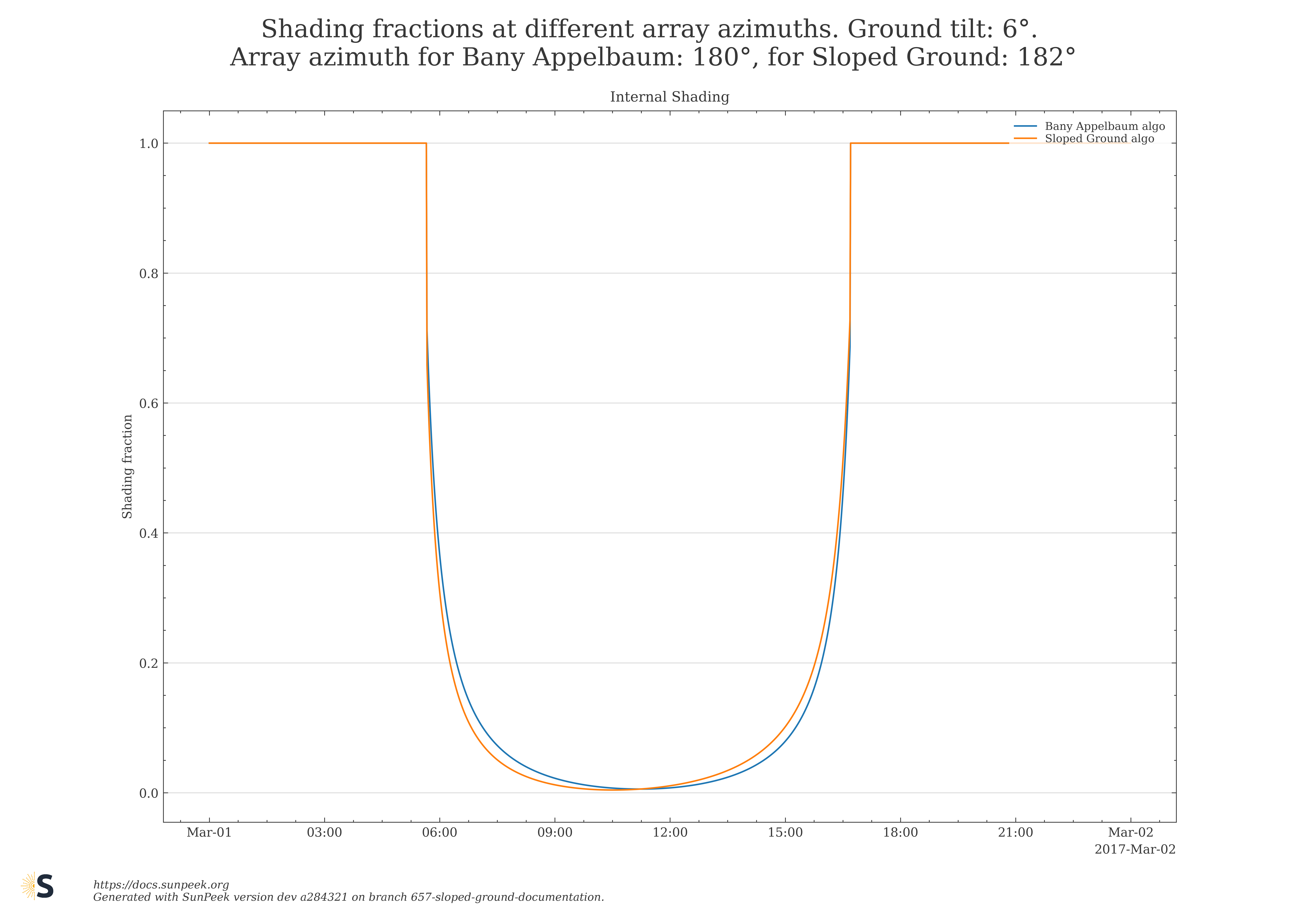
Figure 12: Comparison of shading fractions for slightly deviating collector field azimuths

The last figure shows a comparison of the two algorithms for selected days for a specific configuration of ground tilt, collector tilt, ground azimuth and collector field azimuth.

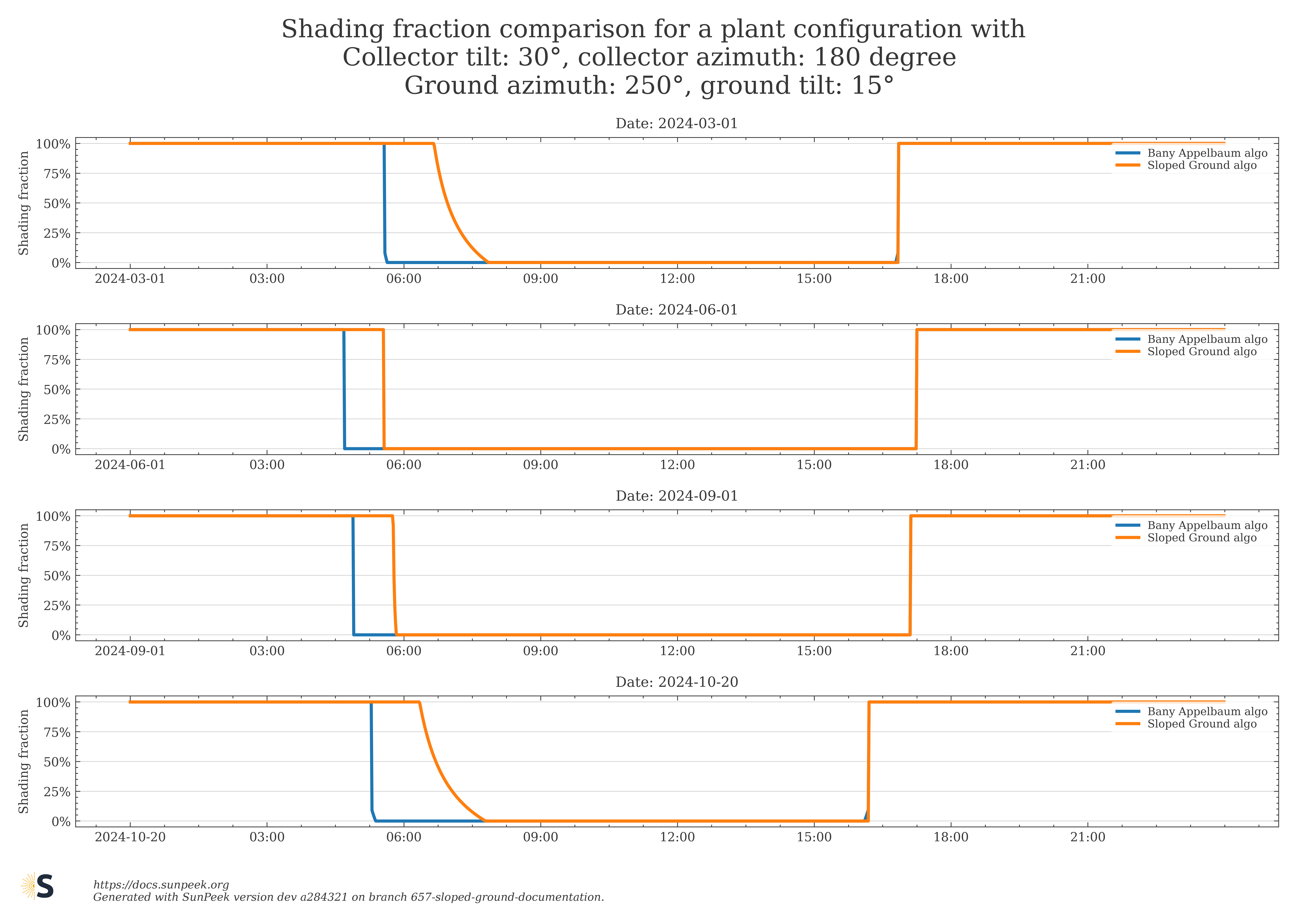
Figure 13: Comparison of both algorithms (Bany Applebaum and new Sloped Ground) for a specific plant configuration