This section tells you how to select a plant if you:
You just created a new plant?
If you followed the tutorial (Adding Plants), the plant you just added is already selected!
Well done! You can continue with the next step (Overview).
You already created a plant earlier?
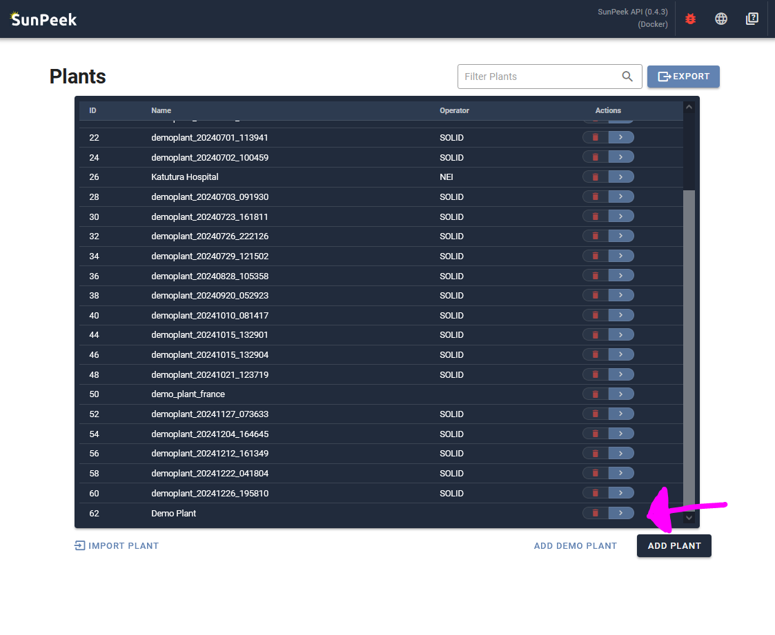
In this case you will see a list of plants when you start SunPeek.
You can either double-click on the desired plant to select it. Or click on the blue edit button on the outer right to select the plant (as shown in the screenshot). You are then redirected to the Overview.
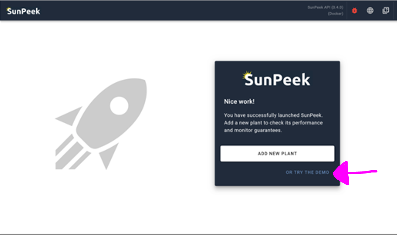
You just started SunPeek?
In this case you will see the SunPeek Welcome Page.
You can either follow the tutorial to add a Adding Plants.
Or you can click on the Try out the Demo button to skip the steps and continue with the pre-configured SunPeek Demo-Plant.
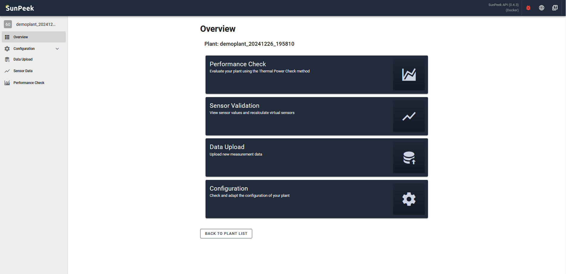
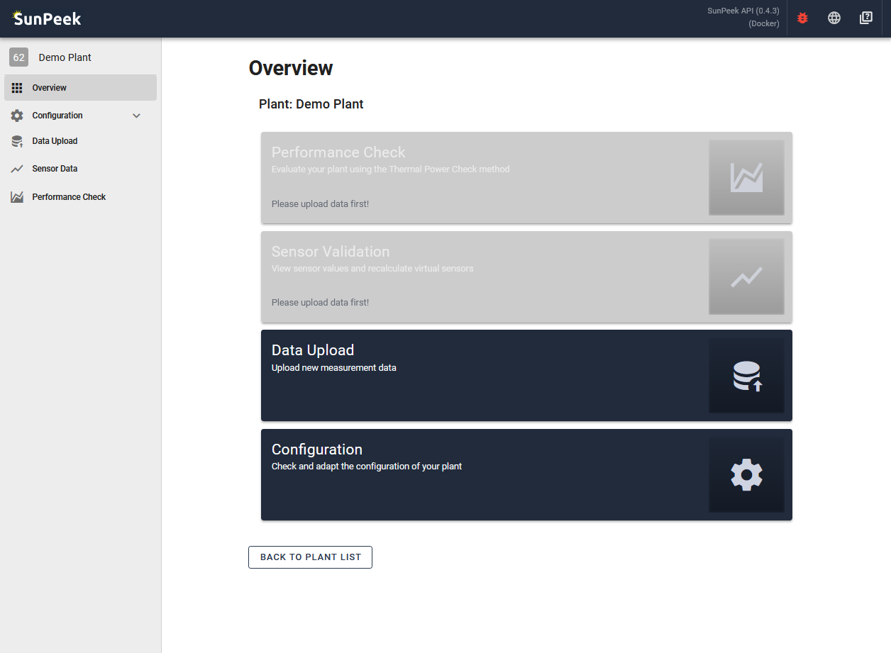
The overview page is shown when you select a plant (Plant Selection).
It provides buttons to visit other pages (as alternative to the navigation bar on the right),
with a short explanation on what can be done on the respective page.
In addition, it also informs the user in case some steps are still missing to run Power Check.
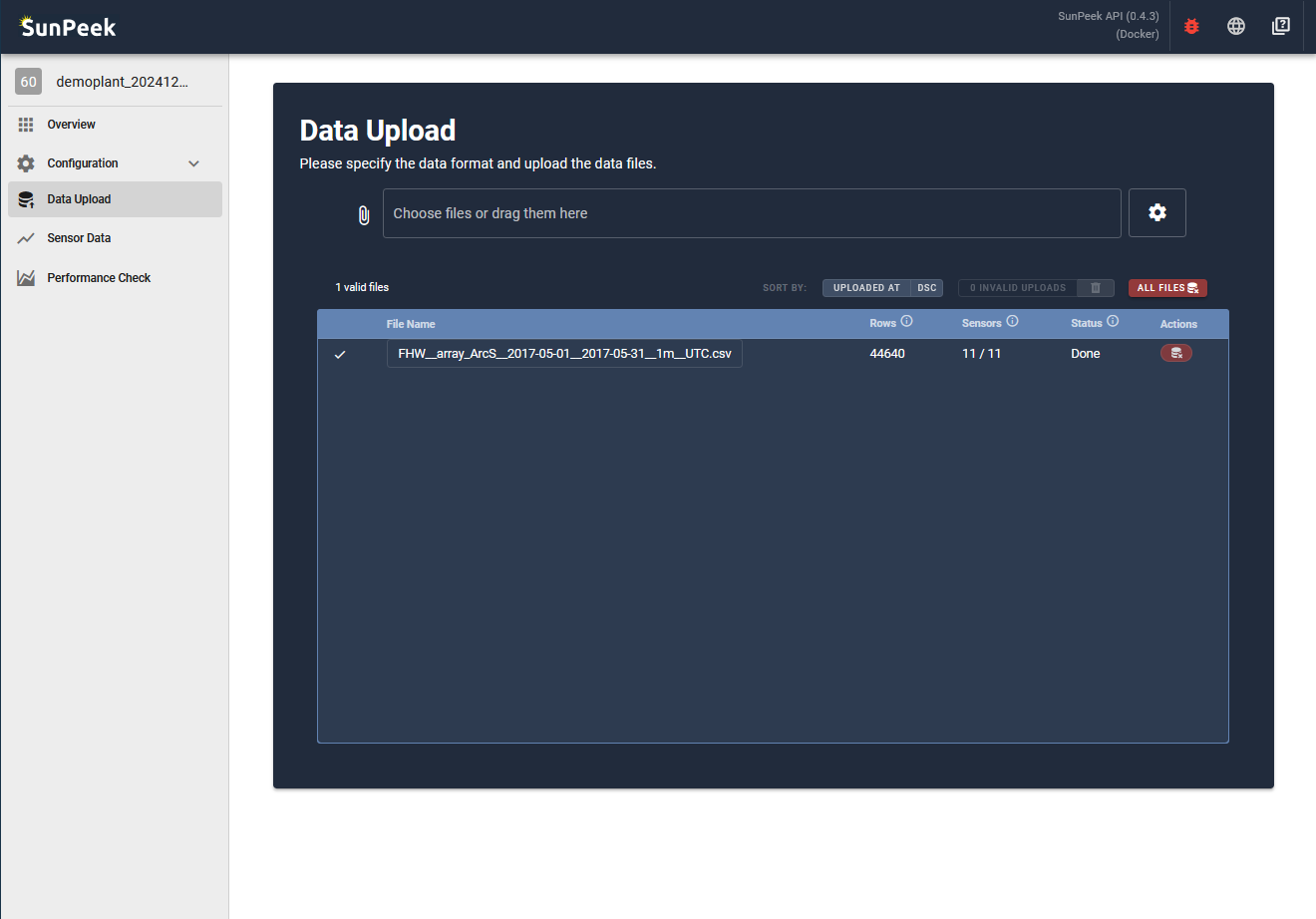
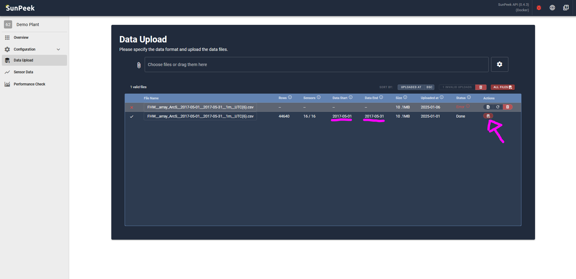
The Data Upload page allows users to upload data to SunPeek.
The data is then stored within the SunPeek database so it can be retrieved fast on demand.
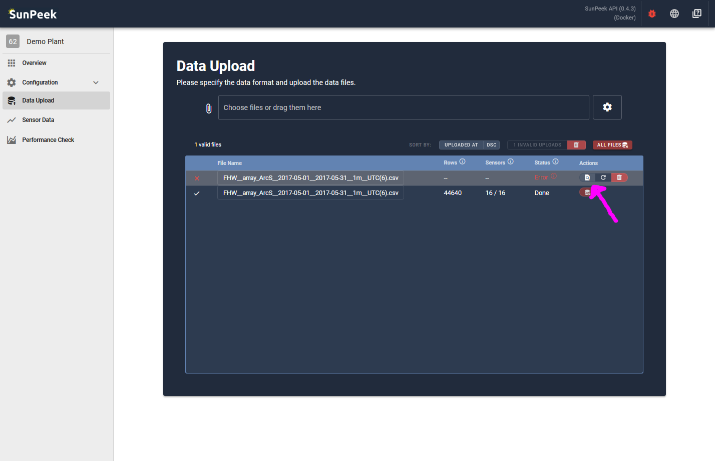
Once data has been uploaded, every uploaded file will appear in the list, as shown in the screenshot above.
The page provides the following information for each uploaded file:
Name
Description
File-Name
The name of the file that was uploaded
Rows
The number of rows inside the file = the number of timestamps in the file
Sensors
The number of sensors identified in the columns of the file, compared to the known sensors based on the sensor information (Sensor Details).
Data Start
Minimum timestamp inside the provided data
Data End
Maximum timestamp inside the provided data
Size
Size of the file
Uploaded at
Time of upload (server time)
Status
The status of the upload:
Done: The data was successfully uploaded
Sending: The WebUI is sending the data to the backend
Parsing: The backend has received the data and is parsing it
Error: There has been an error during upload -> Hover to inspect.
Actions
Provides buttons to delete a file (deletes data between start and end date of the file) and inspect it (only if recently uploaded)
you can use this file here which contains 1 month of FHW data.
and simply drag and drop the file in the file-input
UPLOADING
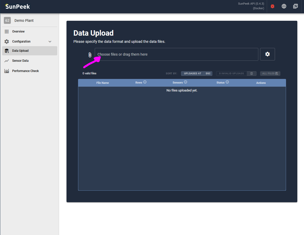
If you have not uploaded any data yet, the list will show “No files uploaded yet”.
In this case you can simply drag and drop a file, or click on the file-input at the top to select a CSV file.
This file should ideally match the format you specified during the data-format step in the configuration (Data Format),
(see further below to adapt the data format)
PARSING
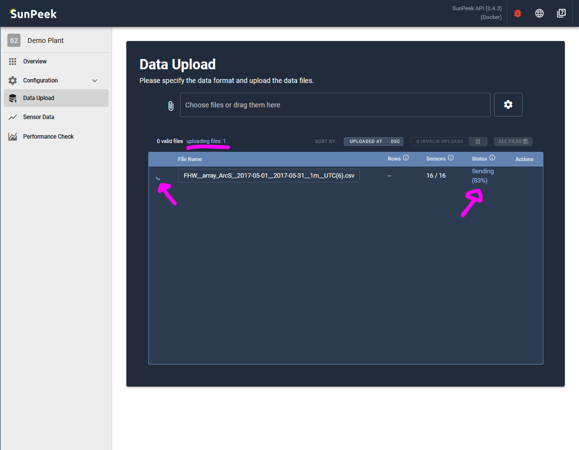
Upon selecting a file, the upload will start:
Sending: First, the data will be sent from the browser to the SunPeek Backend.
Parsing: Next, the backend will parse the data and check if everything is ok.
Error: If there is an error, the upload is terminated without storing any data (see section further below).
Done: Finally, (if there is no error) the data will be saved in the database for easy retrieval and further use.
After this, everything is ready to inspect the uploaded data (Sensor Data) and run Power Check (Run Power Check).
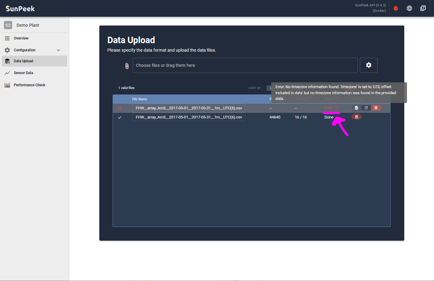
If any problem arises during uploading a file, SunPeek will stop and show Error as the Status of the upload.
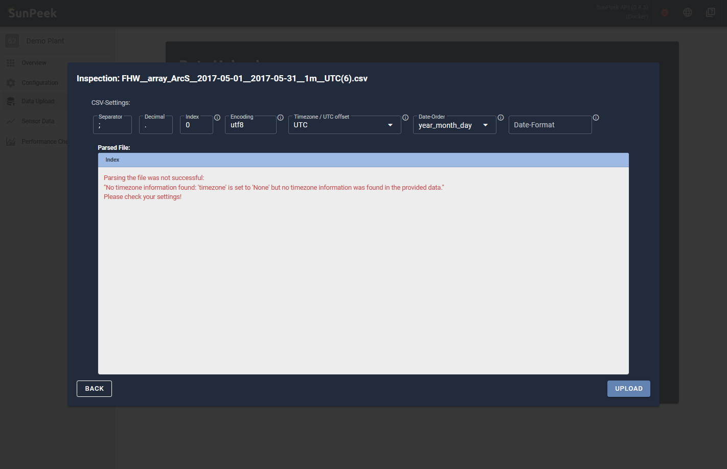
By hovering over the red error symbol, you can find out more details about why the upload failed.
(In the case shown in the screenshot, the date format of the file does not match with the settings and SunPeek cannot understand the timestamps)
If you just uploaded the file (so it’s still available in the browser memory)
you can use the inspect button to inspect the file,
or you can click on the retry button to try to upload the file again.
If you click on inspect you will be able to see the parsed file and the error message in its own window overlaying the data upload.
Typically, you might need to change some data format settings (e.g. if your data logging has changed).
Or you might need to check your file manually (e.g. Notepad++) in case some lines are formatted incorrectly (e.g. missing header in file, bad encodings, etc.).
See also
For more common errors and how to resolve them, see Troubleshooting.
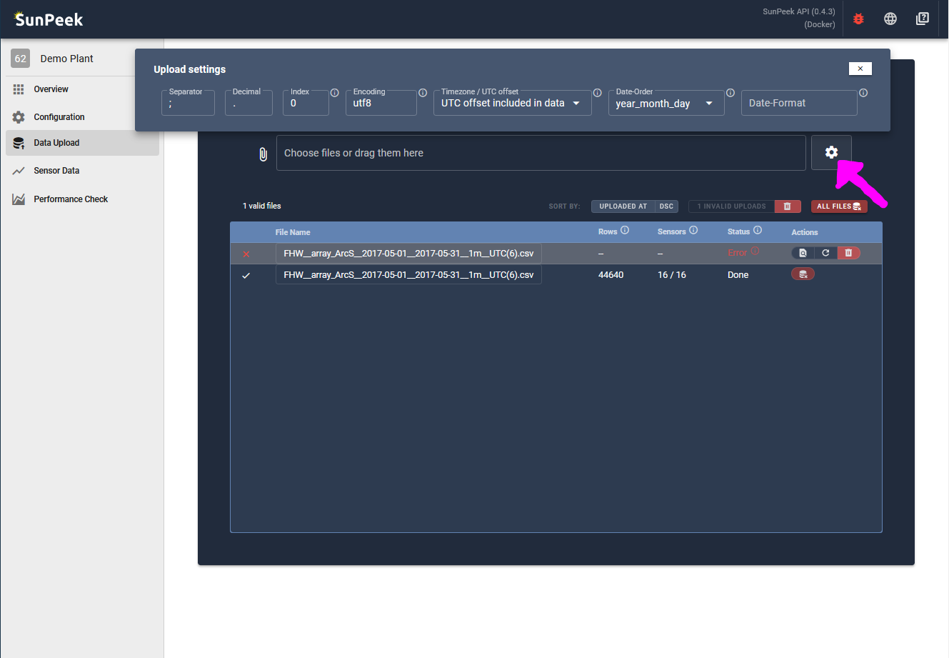
Solar thermal plants have quite a long lifetime, so it is possible that the data logging format might change over time.
In this case, it is easy to adapt the data format by clicking on the gear-icon next to the file-input.
For a detailed explanation of all data format options (separator, decimal, timezone, encoding, etc.),
see Data Format.
Deleting data will only affect the measurement data.
The plant configuration, however, will not be deleted.
Hence, you can simply drag-and-drop files again to re-upload the measurement data.
Mistakes can happen - so it’s important that data can be deleted again, in case a bug occurred or the wrong file was
provided to the SunPeek data upload.
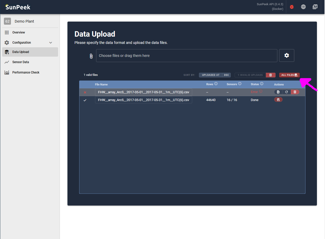
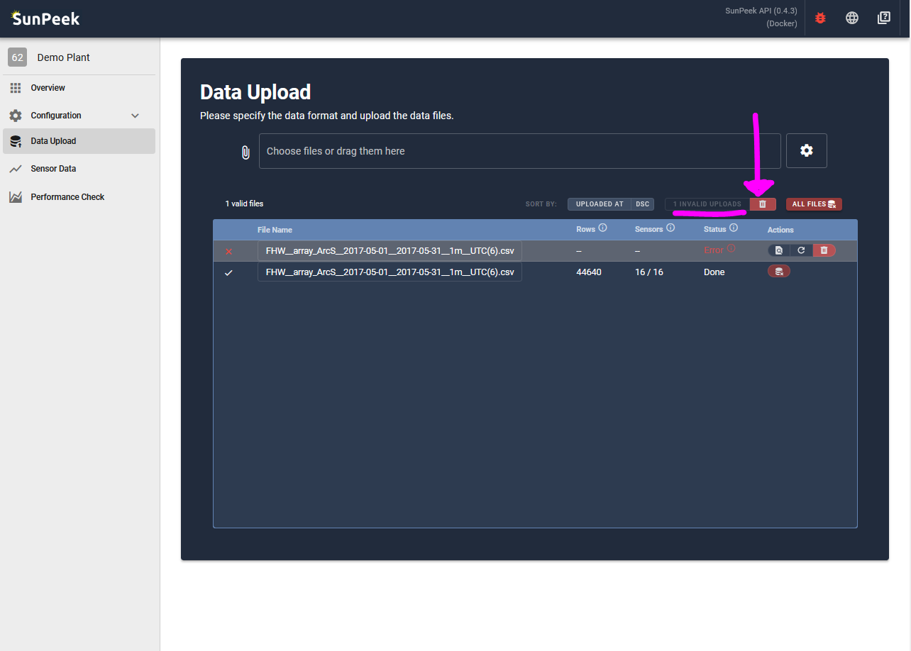
Hence, SunPeek provides ways to delete data either completely or file-by-file.
Delete all data
Clicking on the red All Files button, will delete all measurement data in the SunPeek database,
and also remove the information about which files have been uploaded.
This option can be a good choice if for some reason the whole database is corrupted
(e.g. if you just started uploading and want to start afresh; if you have uploaded a file with incorrect datetime-format and the timestamps are now scattered across multiple months or years)
Delete one file
Alternatively, you can also delete measurement data on file-by-file basis.
For this, SunPeek uses the parsed Start Date and End Date of the file and deletes all the data inbetween.
Hence, in the example in the screenshot above, SunPeek would delete all data between 01.05.2017 and 31.05.2017.
Delete invalid file entries
Invalid Files are files that could not get parsed - resulting in an Error.
Note that in this case no data was uploaded to the database to begin with
This is also reflected by the Data Start and Data End columns, which show no values.
Hence, clicking on the delete-Button for an invalid file will only remove the file-entry, but does not remove measurement data.
For convenience, you can also click the trashcan symbol on the toolbar above the list to delete all invalid file entries.
Again, this will not delete any actual data.
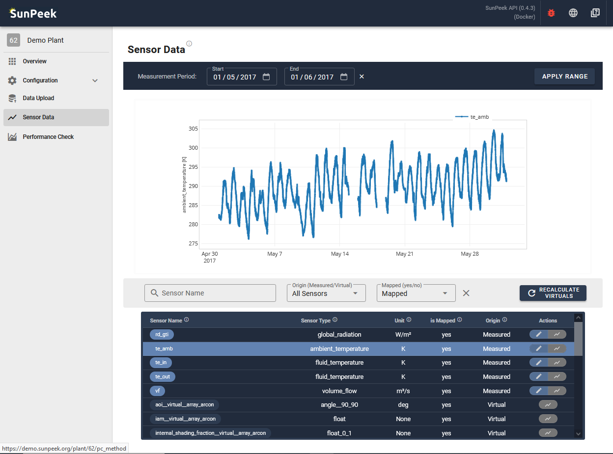
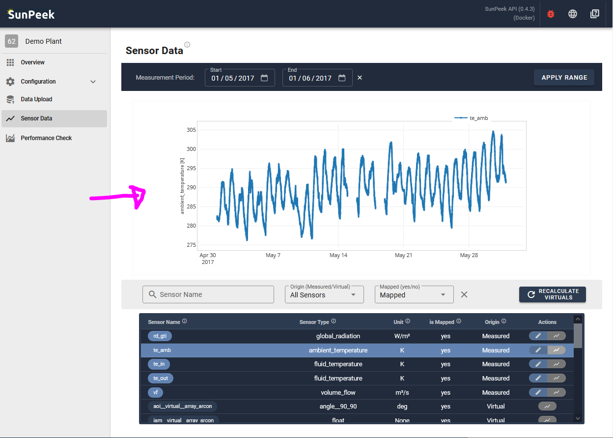
The Sensor Data page allows users to inspect the data that was uploaded to SunPeek.
It can provide a quick check if the sensors were parsed correctly by displaying the measurement values.
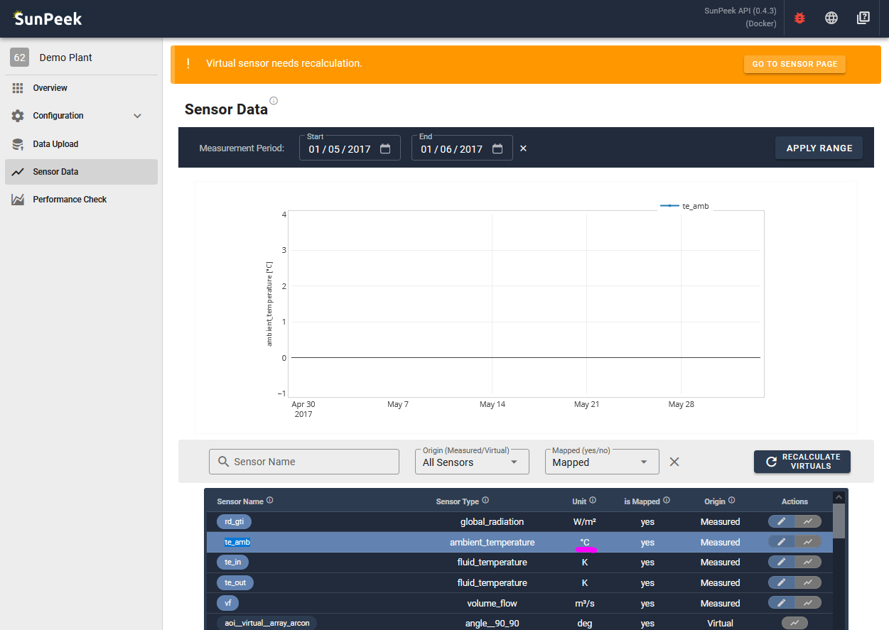
In addition to the measured sensors it can also show the values of the calculated virtual sensors.
The lower half of the screen shows a list of all sensors that are known to SunPeek.
In addition, it also contains virtual sensor - which are sensors that are not provided with the measured data via the data upload, but are calculated inside SunPeek.
For each of the sensors, the name, sensor_type, unit and some other information is displayed in the list.
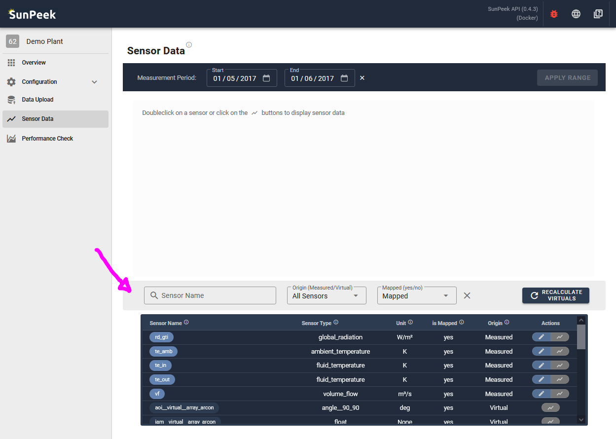
Use the Actions at the right of each sensor, to edit the sensor information (pencil symbol), or to display the data (line chart symbol).
Alternatively, double-clicking on a sensor also shows the measurement data.
A toolbar at the top filters the sensors shown below.
Users can search by name, toggle between virtual or measured sensors, or filter to only show sensors that are mapped within SunPeek.
In addition, the Recalculate Virtuals button recalculates of virtual sensors (which is normally done after uploading data)
Sensor Values
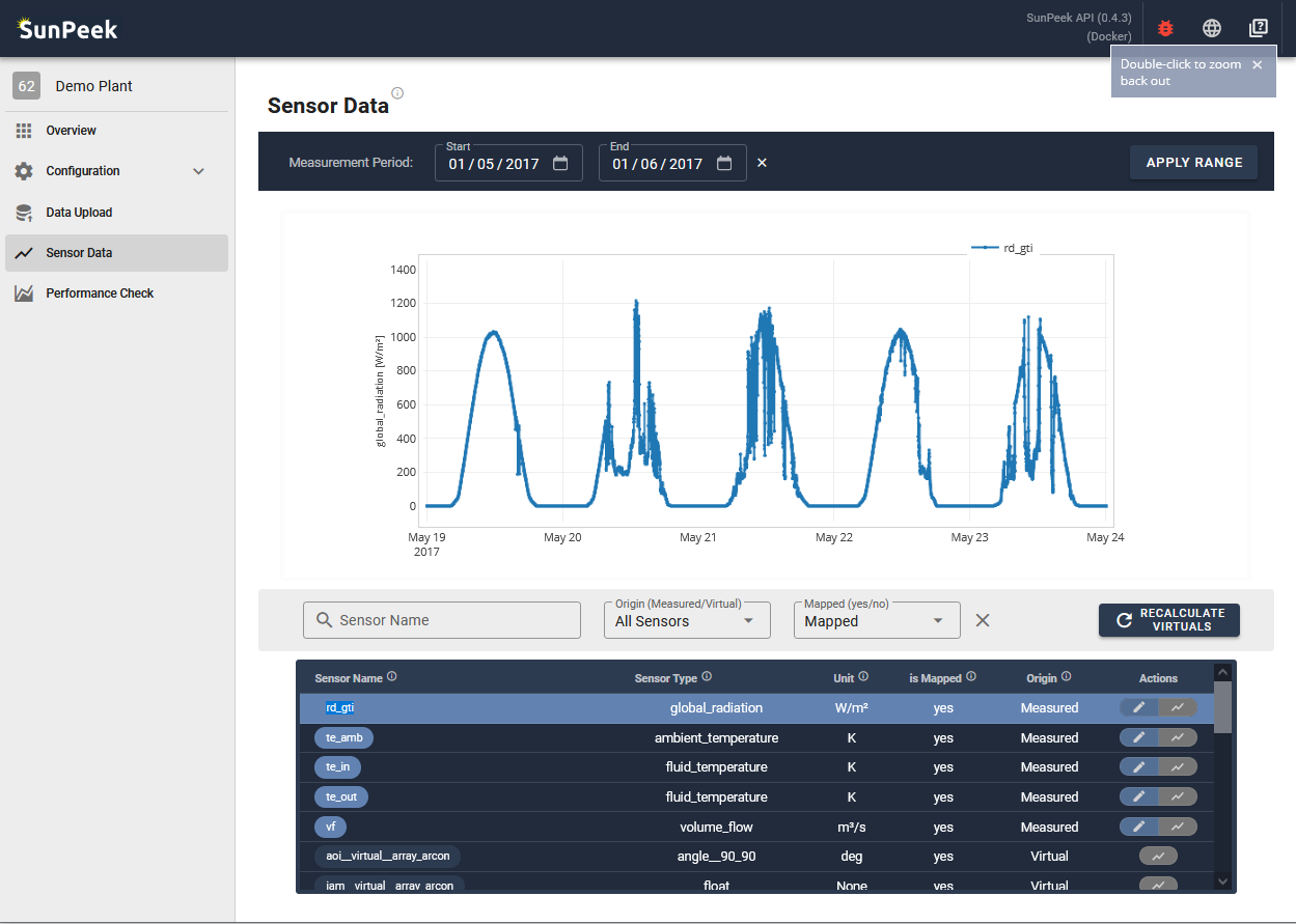
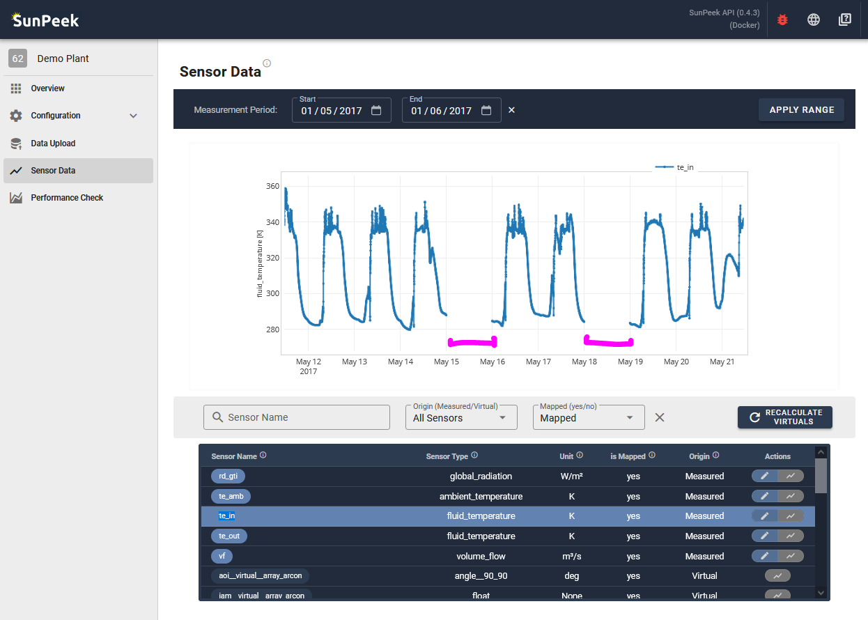
The top of the screen shows the measurement data of a selected sensor as a time chart.
Hover over the values to show more details, and click and drag on the data to zoom.
Double-click on the screen to zoom back out.
In addition, a toolbar above the plot allows to change the time-period that is shown within the plot.
There are multiple use cases how this page might be of help.
Check that the data was imported correctly
After the import it can make sense to make a quick check if the data was imported correctly.
You can randomly select some sensors to see if the values look ok:
Is the unit correct?
Check if the values displayed in the graph match with the unit.
In some cases, the graph will show no data if the sensor readings are labeled as out-of-range
(e.g. ambient temperature of 300K is ok, but 300°C would result in a NAN value).
To adapt the unit, you can click on the edit button on the right.
If you find that a virtual sensor has a wrong unit, it means that one of the sensors used as input has an incorrect unit.
Is the pattern correct?
Check if the pattern of the data matches with your expectation (e.g daily pattern for irradiation).
If not, it could mean the timestamps are not parsed correctly, or the sensor might show abnormal readings.
Are there any large gaps?
If yes, it could mean that part of the data could not be parsed either because it was not available to begin with,
or it contains unknown symbols, or the values are outside the expected range for that type of sensor (e.g. 100°C for ambient temperature).
See also
For details on how SunPeek handles data quality checks, tolerance ranges, and
data replacement schemes, see Data Handling.
Inspect a specific sensor
In case of errors during the execution of Power Check (Run Power Check)
the error message will give you hints about which sensor values are missing or incorrect.
With this information you might come back to the Sensor Data page
to inspect the measurement data of the corresponding sensor.
Alternatively, you might locate outliers in Power Check results which you want to investigate.
In this case, you might click on a few related sensors (that are mapped) and zoom into the time-period where the outlier appeared.
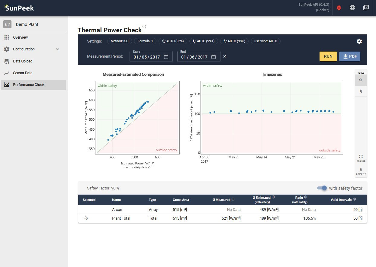
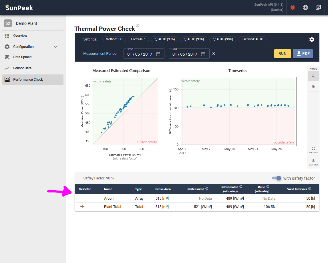
The Power Check page allows users to run Power Check based on the uploaded data.
Here you can set Power Check settings (like safety factors and other parameters) and visualize Power Check results.
Note
For more information on the Power-Check method itself, please check out
The Power Check FAQ, answering some common questions about Power Check.
The top of the page shows the toolbar containing all settings to run Power Check.
In the first row, it displays the Power Check settings that are currently used.
Clicking on a setting or the gear symbol on the right, an overlay appears where you can change the settings (see further below).
If adapted, the settings are saved to the database as well.
The second row contains an input field for specifying the start and end of the measurement period that should be used for the results.
By default, the full known range of the measurement data is used. However, users might want to specify smaller timeframes to speed up the execution.
At the right end of the second row, the toolbar contains two buttons to execute Power Check.
RUN: executes Power Check and displays the information in the Web Interface in interactive plots.
PDF: executes Power Check and downloads a PDF report of Power Check results.
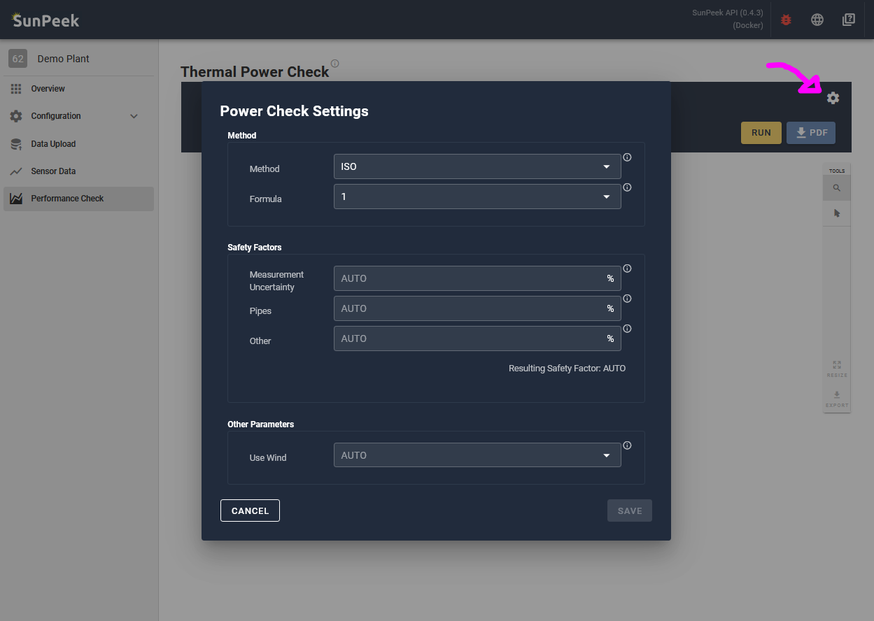
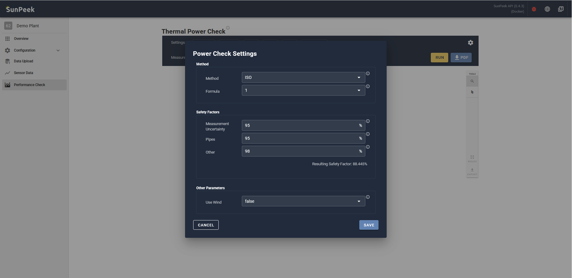
Settings Overlay
Clicking on a setting or the gear symbol on the right,
an overlay appears where you can change the settings:
Method -
the first entry sets the computation method for the results:
ISO - performs Power Check with 1h intervals starting at full hours (as defined in ISO 24194)
Extended - performs Power Check with 1h intervals starting at an arbitrary timestamp. This will increase the number valid timestamps found.
Formula -
selects the formula for Power Check.
AUTO - automatically selects Power Check formula that works best based on the sensor mapping.
1 - only uses the Formula 1 to compute the results.
2 - only uses the Formula 2 to compute the results.
3 - only uses the Formula 2 to compute the results.
Safety factors -
sets individual safety factor values. Using AUTO some default safety factors will be used.
Use Wind -
specifies whether wind speed should be considered or ignored:
true - Power Check will use the wind speed and will fail if not set
false - Power Check will not use wind speed (even if a measurement slot would be available)
AUTO - will select true or false depending whether wind speed is available as a measurement slot (=mapped sensor)
Tip
For more information on how to set the values,
please check the ISO24194 and the Guide to ISO 24194 (Link).
Interactive Results
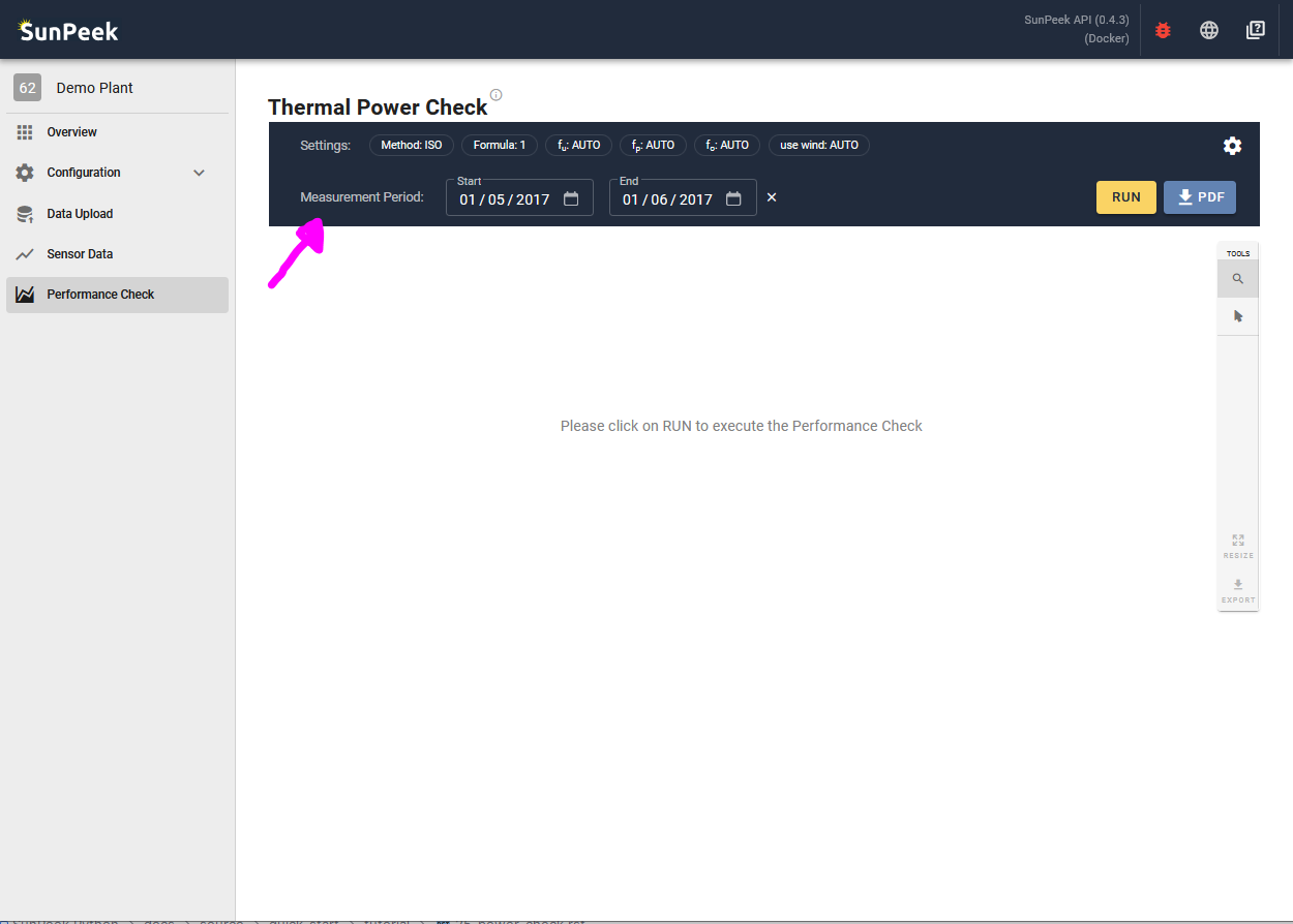
Clicking on the RUN Button, Power Check algorithm is executed.
After calculation, the results will be displayed in the Web-Interface.
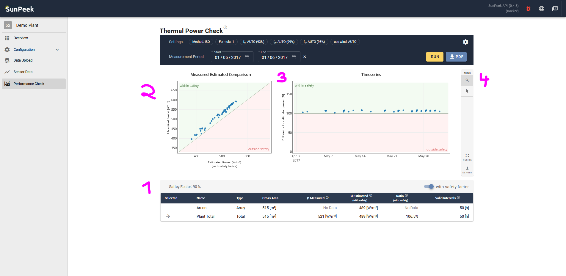
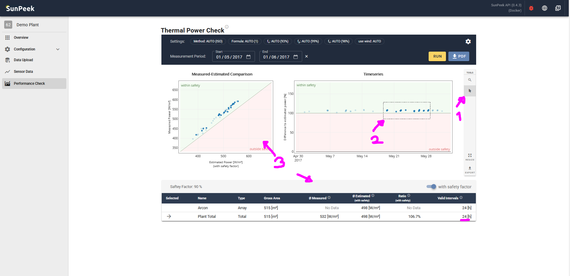
The results page consists of 4 parts:
1. Results Table
The table contains the condensed information about the results - for each collector field (as specified in the configuration) and for the overall plant.
By clicking on a row, the corresponding data is shown in the other plots (2, and 3) as well.
The table displays the following information:
Selected - shows which of the rows is currently selected in the other plots
Name - shows the name of the component (either overall plant or name of the collector array).
Type - shows the type of the component (either overall plant or Array)
Gross Area - shows the gross area of the component
Measured - shows the average measured performance of the component within the valid intervals
Estimated - shows the average estimated performance of the component within the valid intervals
Ratio - shows the ratio of measured to estimated performance of the component within the valid intervals
Valid Intervals - shows the number of valid intervals found within the measurement data.
Note that there is a switch button on top of the table on the outer right which allows you to show the data without safety factor.
2. Measured Estimated Comparison Plot
The Measured-Estimated Comparison Plot shows the results of the selected component in a x-y plot.
Each point in the diagram is a valid interval that has been detected in the data.
The x value shows the estimated power (by default including the safety factor), while the y-Axis shows the measured power within the intervals.
Hence:
if points lie exactly on the diagonal, it means that the estimated and measured performance of the valid interval matches exactly.
if points lie above the diagonal, it means that the measured power is higher than the estimated power of the valid interval.
if points lie below the diagonal, it means that the measured power is lower than the estimated power of the valid interval.
Hence, if the safety factors are set correctly, you would expect the points within the green area above the diagonal,
while points below the diagonal would indicate a collector performance below expectations.
Note that there might be various reasons for underperformance:
incorrect settings (e.g. safety factors or incorrect sensor units)
bad plant operation (e.g. pumps not running, no volume flow)
decreasing plant performance (e.g. accumulating dirt on collector)
low plant performance (e.g. damages)
…
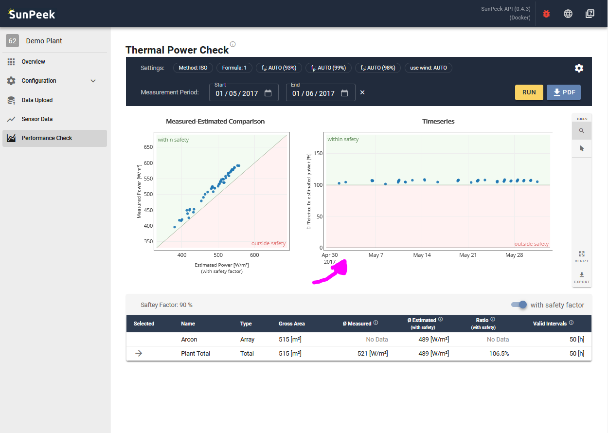
3. Timeseries Plot
The timeseries plot shows results versus time.
This is especially interesting to see any changes in plant performance over the lifetime of the plant.
Again, each point represents one of the valid intervals within the measurement data.
On the y-axis it shows the ratio of measured to estimated power.
Hence, values above 100% means that the measured performance is above the estimated performance.
The representation versus time sometimes allows to give more insights about the plant and Power Check results:
Deteriorating Performance (slow decrease)
In case dust accumulates on the collectors, the performance initially will be very good, but gradually getting worse.
This can be identified with this plot, as you will see a slow decrease of collector performance versus time.
Collector Cleaning (sudden increase)
Assuming a dirty collector, a collector cleaning might increase the performance of the plant again.
Hence, after cleaning, the plot might indicate a sudden increase of the measured-estimated ratio,
with the collector producing more energy again.
Broken sensor (sudden change)
With a broken sensor used for Power Check calculation, results might be wrong.
Hence, if a sensor break occurs, there might be sudden changes in the ratio reported by Power Check.
No pump running (sudden drop)
If the pumps are not running even though irradiation is high, Power Check might still yield results [*].
In such a case, the measured power will be zero as there is no volume flow.
Hence, the ratio of measured to estimated will be close to 0% for times
when pumps are not running despite high irradiation.
Internal-Shading (no points in timeframe)
Power Check prohibits including intervals where collectors are shaded.
Hence, some time periods will not show any valid intervals (e.g. during Winter with low sun).
(unaccounted) External Shading (yearly patterns)
In case of external shading the collector performance is lower compared to unshaded timeperiods.
If the information is not applied to SunPeek (through the is_shaded sensor slot),
Power Check will yield lower ratio of measured to estimated in times where unaccounted external shading occurs.
This may result in seasonal pattern in Power Check results.
[*] see discussion in Guide to ISO 24194 (Link) for more information about stagnation and “no pump running”
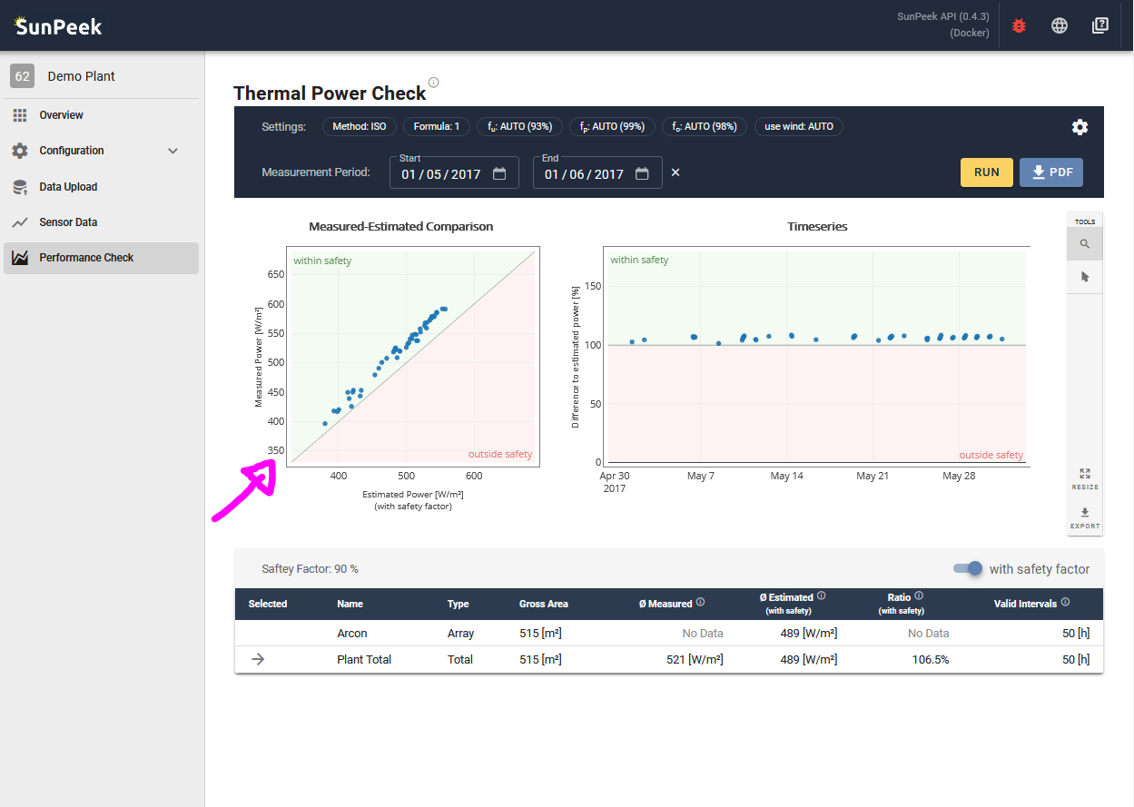
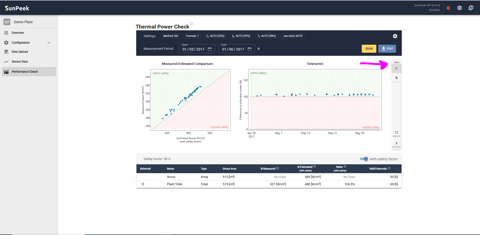
4. Tools
Finally, there is a small toolbar at the outer right of the plots.
TOOL: Zooming - when selected, click and drag over the plots to zoom into the selected area. Doubleclick to reset to the original zoom.
TOOL: Selecting - when selected, click and drag over the valid intervals in the plot to select them. As a result, the same valid intervals will be highlighted in the other plots as well, and the results in the table will adapt.
BUTTON: RESIZE - resets the zoom to the initial zoom.
BUTTON: EXPORT - exports Power Check results as CSV data.
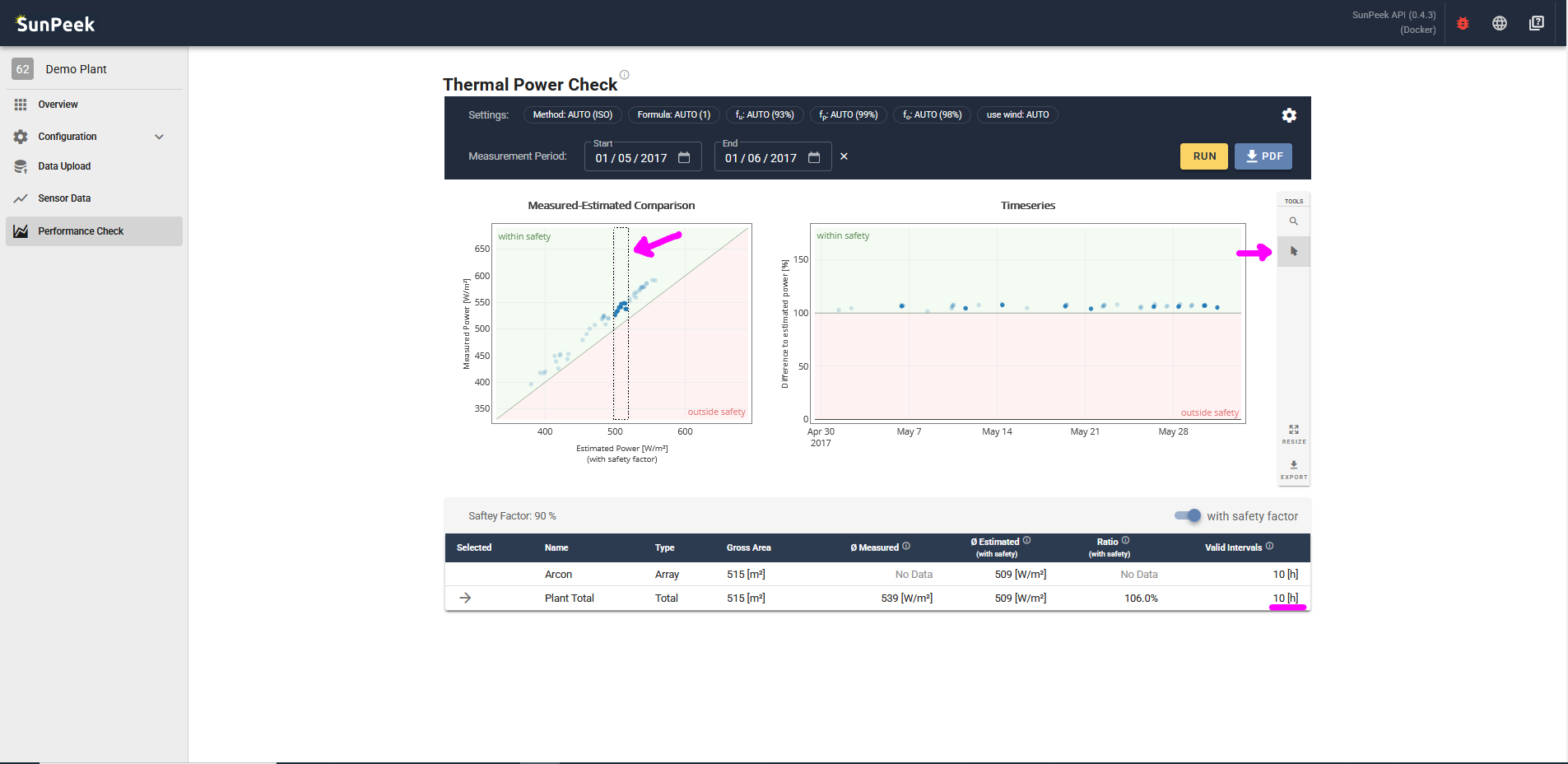
Example 1 - selecting time
Here you can see an example of the selection.
First, select the Selection tool from the toolbar.
Next, select a specific area for example in the timeseries plot.
As a result, the measured-estimated plot and the table will adapt.
Note this could be helpful for example if you only want to know the results of a specific period of time,
or to exclude outlier from the results.
Example 2 - selecting specific section
Here is another example, using the selection tool in the measured-estimated plot.
Again, the timeseries plot and the table will be adapted.
Note this could be helpful for example to see if results change when only taking into account higher measured/estimated power.
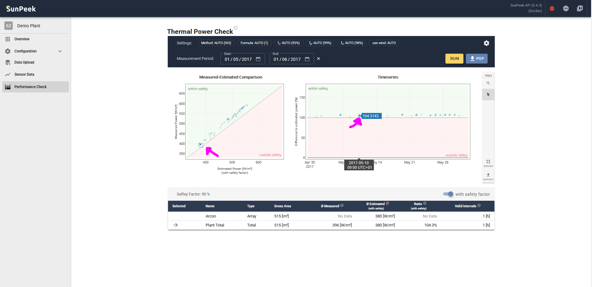
Example 3 - selecting outlier
You can also use the tool to select outlier in the measured/estimated plot and
find out when the outlier happened using the timeseries plot.
In the shown case, we use the selection tool to highlight one valid interval and hover in the timeseries plot to know
when the outlier happened
This assumes you have followed the Tutorial (Adding Plants).
Let’s assume that for this plant there is guarantee between the collector manufacturer, and the plant designer.
As part of the contract, it was agreed upon that Power Check according to ISO 24194 should be used,
to check if the collector performance matches its expectations.
Based on the hydraulics and sensors used, the two parties agreed on the following safety factors:
Measurement Uncertainty: 95%
Pipes: 95%
Other: 99%
In addition, they agreed to use the ISO method as specified in ISO 24194 and use Formula 1 [*].
Unfortunately, there is no wind speed measurement available[*].
However, based on the typical weather of the location, wind speed above 10m/s as specified in ISO is uncommon,
and hence they agree to ignore wind speed in the analysis.
Hence, we adapt the settings accordingly (see screenshot above).
Note
[*] For simplicity, we assumed here that wind speed and beam/diffuse irradiation are not available.
They are in the DEMO dataset, but we haven’t used them in the sensor mapping yet.
Of course, this could be easily adapted without a need to re-upload data.
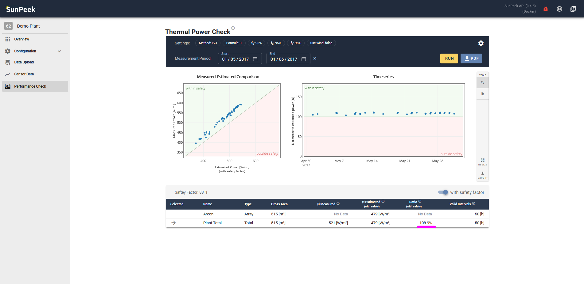
After clicking on RUN, we can see the results of the 1 month performance check (see screenshot above).
In the table, we can see that for the plant, 50 valid intervals have been found.
And in addition, the measured performance during the 50 interval exceeds the estimated performance according to ISO 24194 (including the safety factor).
This is also highlighted in the table with the Ratio showing a value above 100%.
The same can also be seen in the Measured Estimated Comparison and the Timeseries plots.
In all cases, the measured performance is above the estimated one - and inside the green area.
=> Hence, Power Check has been successful - indicating that the collectors perform as expected!